Linear Algebra - Week 4

Dive into the fundamentals of linear algebra for machine learning and data science. This week you’ll learn about eigenvalues and eigenvectors.

from functools import partial
from itertools import product

import matplotlib.pyplot as plt
import numpy as np
import sympy as sp
from IPython.display import display, Math

plt.style.use("seaborn-v0_8-whitegrid")

Eigenvalues and Eigenvectors

Basis

🔑 A basis of a space is a set of linearly independent vectors that spans the space.

In a 1-D space, we can only have one element in the basis; in a 2-D space, we can only have two elements in the basis, and so on.

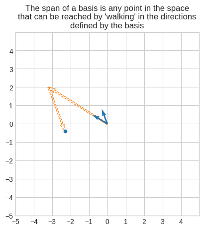
🔑 The span of a basis is the space consisting of all linear combinations of the basis.

Metaphorically, the span of a basis is any point in a space that can be reached by walking only in the directions defined by the basis.

plt.quiver(
    [0, 4 * -0.8, 0, 0],
    [0, 4 * 0.5, 0, 0],
    [
        4 * -0.8,
        -3 * -0.3,
        -0.3,
        -0.8,
    ],
    [4 * 0.5, -3 * 0.8, 0.8, 0.5],
    angles="xy",
    fc=["none", "none", "tab:blue", "tab:blue"],
    ec=["tab:orange", "tab:orange", "none", "none"],
    ls=["dashed", "dashed", "solid", "solid"],
    linewidth=1,
    scale_units="xy",
    scale=1,
)
end_point = np.array([4 * -0.8, 4 * 0.5]) - np.array([3 * -0.3, 3 * 0.8])
plt.scatter(end_point[0], end_point[1], s=20, c="tab:blue")
plt.xticks(np.arange(-5, 5))
plt.yticks(np.arange(-5, 5))
plt.xlim(-5, 5)
plt.ylim(-5, 5)
plt.gca().set_aspect("equal")
plt.title(
    "The span of a basis is any point in the space\nthat can be reached by 'walking' in the directions\ndefined by the basis"
)
plt.show()

Eigenvalues

Let’s consider the following linear transformations:

\(A_1 = \begin{bmatrix}2&&1\\0&&3\end{bmatrix}\)

\(A_2 = \begin{bmatrix}3&&0\\0&&3\end{bmatrix}\)

\(A_3 = \begin{bmatrix}2&&0\\0&&2\end{bmatrix}\)

We can demonstrate that although \(A_1\) and \(A_2\) are different transformations, they are indeed the same for infinitely many points.

And the same can be demonstrated for \(A_1\) and \(A_3\).

A1 = np.array([[2, 1], [0, 3]])
A2 = np.array([[3, 0], [0, 3]])
A3 = np.array([[2, 0], [0, 2]])
e_set = set(product([-1, 0, 1], [-1, 0, 1])) - set([(0, 0)])

fig, (ax1, ax2) = plt.subplots(nrows=1, ncols=2, figsize=(10, 5))
for e in e_set:
    ax1.scatter(e[0], e[1], c="tab:blue")
    ax2.scatter(e[0], e[1], c="tab:blue")
    t_e1 = A1 @ e
    ax1.scatter(t_e1[0], t_e1[1], c="tab:orange", alpha=0.5)
    ax2.scatter(t_e1[0], t_e1[1], c="tab:orange", alpha=0.5)
    t_e2 = A2 @ e
    ax1.scatter(t_e2[0], t_e2[1], c="tab:green", alpha=0.5)
    t_e3 = A3 @ e
    ax2.scatter(t_e3[0], t_e3[1], c="tab:green", alpha=0.5)
ax1.plot([-5, 5], [-5, 5], color="tab:orange", alpha=0.5)
ax1.plot([-5, 5], [-5, 5], color="tab:green", alpha=0.5)
ax2.plot([-5, 5], [0, 0], color="tab:orange", alpha=0.5)
ax2.plot([-5, 5], [0, 0], color="tab:green", alpha=0.5)
ax1.set_xticks(np.arange(-5, 5))
ax1.set_yticks(np.arange(-5, 5))
ax2.set_xticks(np.arange(-5, 5))
ax2.set_yticks(np.arange(-5, 5))
ax1.set_xlim(-5, 5)
ax1.set_ylim(-5, 5)
ax2.set_xlim(-5, 5)
ax2.set_ylim(-5, 5)
ax1.set_aspect("equal")
ax2.set_aspect("equal")
ax1.set_title("$A_1$ and $A_2$ are the same for all the points on the line")
ax2.set_title("$A_1$ and $A_3$ are the same for all the points on the line")
plt.legend(
    ["original", "$A_1$ transformation", "$A_2$ or $A_3$ transformation"],
    bbox_to_anchor=(1.01, 0.99),
)
plt.show()

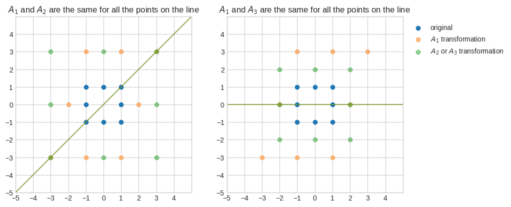
With some imagination, we can see that the blue square on the left-hand side gets sheared horizontally with \(A_1\) and gets blown out with \(A_2\).

We can also see that the points (1, 1) and (-1, -1) go to (3, 3) and (-3, -3) respectively with both \(A_1\) and \(A_2\).

Similarly, the points (1, 0) and (-1, 0) go to (2, 0) and (-2, 0) respectively with both \(A_1\) and \(A_3\).

We can verify that the difference between \(A_1\) and \(A_2\) (and \(A_1\) and \(A_3\)) are singular transformations.

display(
    Math(
        "A_1 - A_2="
        + sp.latex(sp.Matrix(A1 - A2))
        + "A_1 - A_3="
        + sp.latex(sp.Matrix(A1 - A3))
    )
)
assert np.linalg.det(A1 - A2) == 0
assert np.linalg.det(A1 - A3) == 0

$\displaystyle A_1 - A_2=\left[\begin{matrix}-1 & 1\\0 & 0\end{matrix}\right]A_1 - A_3=\left[\begin{matrix}0 & 1\\0 & 1\end{matrix}\right]$

The first system of equations is singular and it has infinitely many solution all of which lie on the line \(y = x\).

\(\begin{cases}-x+y=0\\0x+0y=0\end{cases} = \begin{cases}y=x\\0=0\end{cases}\)

The second system of equations is also singular and it has infinitely many solutions all of which lie on the line \(y = 0\).

\(\begin{cases}0x+y=0\\0x+y=0\end{cases} = \begin{cases}y=0\\y=0\end{cases}\)

It turns out that \(A_2\) and \(A_3\) have the eigenvalues 2 and 3 of the matrix \(A_1\) along their diagonals.

Formally, \(\lambda\) is an eigenvalue of \(A_1\) if

\(\begin{bmatrix}2&&1\\0&&3\end{bmatrix} - \lambda\begin{bmatrix}1&&0\\0&&1\end{bmatrix} = \begin{bmatrix}0\\0\end{bmatrix}\)

or more compactly

\(\begin{bmatrix}2-\lambda&&1\\0&&3-\lambda\end{bmatrix} = \begin{bmatrix}0\\0\end{bmatrix}\)

To find the value(s) of \(\lambda\) we can use the formula for the determinant, and leverage the fact that it must be zero.

\((2-\lambda) \times (3-\lambda) - 1 \times 0 = 0\)

\((2-\lambda) \times (3-\lambda) = 1 \times 0\)

Finally we apply the Zero-Factor Property (if the product of two factors is zero, then at least one of the factors must be zero):

\((2-\lambda) = 0 \Rightarrow \lambda = 2\)

\((3-\lambda) = 0 \Rightarrow \lambda = 3\)

🔑 \(\det(A - \lambda I)\) is called the charateristic polynomial

🔑 The values of \(\lambda\) for which the charateristic polynomial is zero are called roots of the charateristic polynomial

🔑 The eigenvalues are the roots of the charateristic polynomial

So basically, to find the eigenvalues of \(A\) we look at the charateristic polynomial \(\det(A - \lambda I)\) and find the roots, that is we solve \(\det(A - \lambda I) = 0\) for \(\lambda\).

Eigenvectors

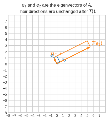
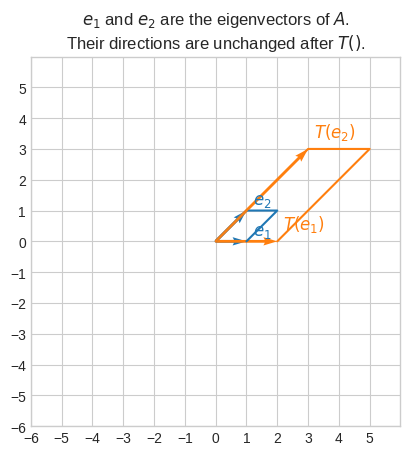
🔑 An eigenvector is any vector whose direction is not changed by a linear transformation and it’s only stretched by the eigenvalues.

Formally, \(\vec{v}\) is an eigenvector of \(A\) if

\(Av = \lambda v\)

This can be rewritten as

\((A - \lambda I)v = 0\)

Note that we express the column vector \(\lambda v\) in matrix form \(\lambda Iv\) when we move it to the left hand side.

Let’s continue the example from the previous section and find the eigenvectors.

We basically need to find \(\vec{v}\) in this system.

\(\begin{bmatrix}2-\lambda&&1\\0&&3-\lambda\end{bmatrix} \begin{bmatrix}v_1\\v_2\end{bmatrix} = \begin{bmatrix}0\\0\end{bmatrix}\)

For \(\lambda=2\) we have

\(\begin{bmatrix}0&&1\\0&&1\end{bmatrix} \begin{bmatrix}v_1\\v_2\end{bmatrix} = \begin{bmatrix}0\\0\end{bmatrix}\).

The coefficient matrix can be converted to the row-echelon form (after \(R2 = R2 - R1\))

\(\begin{bmatrix}0&&1\\0&&0\end{bmatrix} \begin{bmatrix}v_1\\v_2\end{bmatrix} = \begin{bmatrix}0\\0\end{bmatrix}\)

to obtain the following system of equations

\(\begin{cases}v_2=0\\0=0\end{cases}\)

which has solution \(\vec{v} = \langle1, 0\rangle\) or any multiple.

For \(\lambda=3\) we have

\(\begin{bmatrix}-1&&1\\0&&0\end{bmatrix} \begin{bmatrix}v_1\\v_2\end{bmatrix} = \begin{bmatrix}0\\0\end{bmatrix}\),

which is already in row-echelon form, so we only need to solve the following system of equations

\(\begin{cases}-v_1+v_2=0\\0=0\end{cases}\)

\(\begin{cases}v_2=v_1\\0=0\end{cases}\)

to find the solution is \(\vec{v} = \langle1, 1\rangle\) or any multiple.

def plot_transformation(T, title, ax, basis=None, lim=5):
    if basis is None:
        e1 = np.array([[1], [0]])
        e2 = np.array([[0], [1]])
    else:
        e1, e2 = basis
    zero = np.zeros(1, dtype="int")
    c = "tab:blue"
    c_t = "tab:orange"
    ax.set_xticks(np.arange(-lim, lim))
    ax.set_yticks(np.arange(-lim, lim))
    ax.set_xlim(-lim, lim)
    ax.set_ylim(-lim, lim)
    _plot_vectors(e1, e2, c, ax)
    ax.plot(
        [zero, e2[0], e1[0] + e2[0], e1[0]],
        [zero, e2[1], e1[1] + e2[1], e1[1]],
        color=c,
    )
    _make_labels(e1, "$e_1$", c, y_offset=(-0.2, 1.0), ax=ax)
    _make_labels(e2, "$e_2$", c, y_offset=(-0.2, 1.0), ax=ax)
    e1_t = T(e1)
    e2_t = T(e2)
    _plot_vectors(e1_t, e2_t, c_t, ax)
    ax.plot(
        [zero, e2_t[0], e1_t[0] + e2_t[0], e1_t[0]],
        [zero, e2_t[1], e1_t[1] + e2_t[1], e1_t[1]],
        color=c_t,
    )
    _make_labels(e1_t, "$T(e_1)$", c_t, y_offset=(0.0, 1.0), ax=ax)
    _make_labels(e2_t, "$T(e_2)$", c_t, y_offset=(0.0, 1.0), ax=ax)
    ax.set_aspect("equal")
    ax.set_title(title)


def _make_labels(e, text, color, y_offset, ax):
    e_sgn = 0.4 * np.array([[1] if i == 0 else i for i in np.sign(e)])
    return ax.text(
        e[0] - 0.2 + e_sgn[0],
        e[1] + y_offset[0] + y_offset[1] * e_sgn[1],
        text,
        fontsize=12,
        color=color,
    )


def _plot_vectors(e1, e2, color, ax):
    ax.quiver(
        [0, 0],
        [0, 0],
        [e1[0], e2[0]],
        [e1[1], e2[1]],
        color=color,
        angles="xy",
        scale_units="xy",
        scale=1,
    )


def T(A, v):
    w = A @ v
    return w


A = np.array([[2, 1], [0, 3]])
evecs = [np.array([[1], [0]]), np.array([[1], [1]])]
lambdas = [2, 3]

for lam, evc in zip(lambdas, evecs):
    assert np.array_equal((A - lam * np.identity(2)) @ evc, np.zeros((2, 1)))
    assert np.array_equal(A @ evc, lam * evc)

fig, ax = plt.subplots()
plot_transformation(
    partial(T, A),
    title="$e_1$ and $e_2$ are the eigenvectors of $A$.\nTheir directions are unchanged after $T()$.",
    ax=ax,
    basis=evecs,
    lim=6,
)

Let’s consider another matrix.

\(A = \begin{bmatrix}9&&4\\4&&3\end{bmatrix}\)

To find the eigenvalues we solve

\((9-\lambda)(3-\lambda)-16=0\)

\(\lambda^2-12\lambda+27-16=0\)

\((1-\lambda)(11-\lambda)=0\)

So the eigenvalues are \(\lambda=1\) and \(\lambda=11\).

For \(\lambda=1\) the eigenvector is given by

\(\begin{bmatrix}8&&4\\4&&2\end{bmatrix} \begin{bmatrix}v_1\\v_2\end{bmatrix} = \begin{bmatrix}0\\0\end{bmatrix}\).

The coefficient matrix can be converted to the row-echelon form (after \(R1 = 0.125R1\), \(R2 = 0.25R2\), \(R2 = R2 - R1\))

\(\begin{bmatrix}1&&0.5\\0&&0\end{bmatrix} \begin{bmatrix}v_1\\v_2\end{bmatrix} = \begin{bmatrix}0\\0\end{bmatrix}\)

to obtain the following system of equations

\(\begin{cases}v_1+0.5v_2=0\\0=0\end{cases}\)

\(\begin{cases}v_1=-0.5v_2\\0=0\end{cases}\)

which has solution \(\vec{v} = \langle-0.5, 1\rangle\) or any multiple.

For \(\lambda = 11\) the eigenvector is given by

\(\begin{bmatrix}-2&&4\\4&&-8\end{bmatrix} \begin{bmatrix}v_1\\v_2\end{bmatrix} = \begin{bmatrix}0\\0\end{bmatrix}\).

The coefficient matrix can be converted to the row-echelon form (after \(R1=-0.5R1\), \(R2=-0.5R2\) and \(R2 = R2 - R1\))

\(\begin{bmatrix}1&&-2\\0&&0\end{bmatrix} \begin{bmatrix}v_1\\v_2\end{bmatrix} = \begin{bmatrix}0\\0\end{bmatrix}\)

to obtain the following system of equations

\(\begin{cases}v_1-2v_2=0\\0=0\end{cases}\)

\(\begin{cases}v_1=2v_2\\0=0\end{cases}\)

which has solution \(\vec{v} = \langle2, 1\rangle\) or any multiple.

A = np.array([[9, 4], [4, 3]])
lambdas = [1, 11]
evecs = [np.array([[-0.5], [1]]), np.array([[0.5], [0.25]])]

for lam, evc in zip(lambdas, evecs):
    assert np.array_equal((A - lam * np.identity(2)) @ evc, np.zeros((2, 1)))
    assert np.array_equal(A @ evc, lam * evc)

fig, ax = plt.subplots()
plot_transformation(
    partial(T, A),
    title="$e_1$ and $e_2$ are the eigenvectors of $A$.\nTheir directions are unchanged after $T()$.",
    ax=ax,
    basis=evecs,
    lim=8,
)