Calculus - Extra curriculum

Dive into the fundamentals of calculus for machine learning and data science. This week you’ll learn about the Lagrange multiplier method and Quasi-Newton Methods like BFGS. We’ll also revisit linear algebra and calculate the direct inverse of the Hessian matrix for the BFGS update.

import re
from collections import ChainMap
from itertools import combinations

import cvxopt
import matplotlib.pyplot as plt
import numpy as np
import plotly.graph_objects as go
import plotly.io as pio
import sympy as sp
from IPython.core.getipython import get_ipython
from IPython.display import display, HTML, Math
from matplotlib.animation import FuncAnimation
from shapely.geometry import LineString, Polygon

plt.style.use("seaborn-v0_8-whitegrid")
pio.renderers.default = "plotly_mimetype+notebook"

Lagrange multiplier method

🔑 The method of Lagrange multiplier is a method of finding the local minima or local maxima of a function subject to equality or inequality constraints

Let’s say we want to find the maximum or minimum of \(f(x, y) = 5x - 3y\) subject to the constraint \(g(x, y) = 136\) where \(g(x, y) = x^2 + y^2\).

A constrained minimization problem \(\textbf{P}\) would be expressed as

\(\begin{array}{l} \textbf{P} \\ \min \limits_{x,y} 5x - 3y \\ \text{subject to} \quad x^2 + y^2 = 136 \end{array}\)

x, y = sp.symbols("x, y")
f = 5 * x - 3 * y
g = x**2 + y**2

x_ = np.linspace(-15, 15, 250)
y_ = np.linspace(-15, 15, 250)
xx, yy = np.meshgrid(x_, y_)

fig, ax = plt.subplots()
cs1 = ax.contour(
    xx, yy, sp.lambdify((x, y), f, "numpy")(xx, yy), levels=20, cmap="RdBu_r"
)
cs2 = ax.contour(
    xx, yy, sp.lambdify((x, y), g, "numpy")(xx, yy), levels=[136], colors="k"
)
ax.clabel(cs1, inline=True, fontsize=10)
ax.clabel(cs2, inline=True, fontsize=10)
ax.spines[["left", "bottom"]].set_position(("data", 0))
ax.text(1.02, 0, "$x$", transform=ax.get_yaxis_transform())
ax.text(0, 1.02, "$y$", transform=ax.get_xaxis_transform())
ax.set_xlim(-15, 15)
ax.set_ylim(-15, 15)
ax.set_aspect("equal")
plt.title("Contour plot of $f(x, y)$ with constraint $g(x) = 136$", pad=20.0)
plt.show()

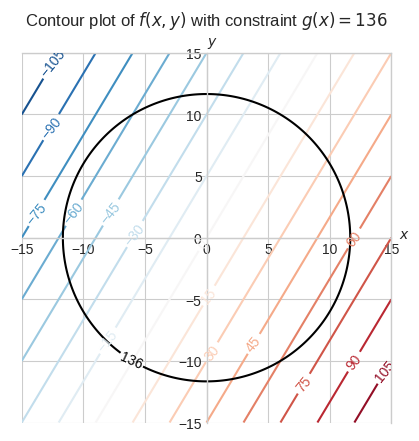
The plot above might not make a lot of sense at a first glance. To hopefully gain a better intuition let’s consider a different visualization.

f_values = sp.lambdify((x, y), f, "numpy")(xx, yy)
f_surface = go.Surface(
    z=f_values,
    x=xx,
    y=yy,
    colorscale="RdBu_r",
    contours=dict(z=dict(start=-105, end=105, size=15, show=True)),
    colorbar=dict(title="f(x, y)"),
    name="f(x, y)",
)

g_values = sp.lambdify((x, y), g, "numpy")(xx, yy)
mask = np.isclose(g_values, 136, atol=5.0)
z_masked = f_values.copy()
x_masked = xx.copy()
y_masked = yy.copy()
z_masked[~mask] = np.nan
x_masked[~mask] = np.nan
y_masked[~mask] = np.nan

g_constraint = go.Scatter3d(
    z=z_masked.flatten(),
    x=x_masked.flatten(),
    y=y_masked.flatten(),
    marker=dict(color="#000000", size=1),
    showlegend=False,
    name="g(x, y)",
)

fig = go.Figure([f_surface, g_constraint])
fig.update_layout(
    title="f(x, y) with projected constraint g(x) = 136 onto it",
    autosize=False,
    width=600,
    height=600,
    scene_aspectmode="cube",
    margin=dict(l=10, r=10, b=10, t=30),
    scene_camera=dict(
        eye=dict(x=-1.8, y=1.4, z=0.7),
    ),
)
fig.show()

\(f(x, y)\) is a linear function so its minimum and maximum are \(-\infty\) and \(+\infty\) respectively.

The constraint bounds its minimum and maximum to values such that \(x\) and \(y\) lies within the circle \(x^2 + y^2\).

If we hover the cursor over the boundary of the constraint, where the surface has the deepest blue possible, we’ll find the minimum of this constrained problem which is around -68.

The contour plot we saw earlier with just the contour of \(f(x, y) = -68\) gives an insight of how we can solve this problem analytically.

_, ax = plt.subplots()
cs1 = ax.contour(
    xx, yy, sp.lambdify((x, y), f, "numpy")(xx, yy), levels=[-68], cmap="RdBu_r"
)
cs2 = ax.contour(
    xx, yy, sp.lambdify((x, y), g, "numpy")(xx, yy), levels=[136], colors="k"
)
ax.clabel(cs1, inline=True, fontsize=10)
ax.clabel(cs2, inline=True, fontsize=10)
ax.spines[["left", "bottom"]].set_position(("data", 0))
ax.text(1.02, 0, "$x$", transform=ax.get_yaxis_transform())
ax.text(0, 1.02, "$y$", transform=ax.get_xaxis_transform())
ax.set_xlim(-15, 15)
ax.set_ylim(-15, 15)
ax.set_aspect("equal")
plt.title("Contour plot of $f(x, y)=-68$ with constraint $g(x) = 136$", pad=20.0)
plt.show()

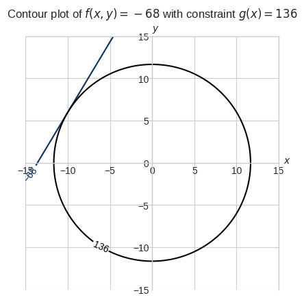
The contour \(f(x, y) = 68\) is tangent to the contour \(g(x, y) = 136\).

It turns out there is an interesting geometric interpretation of the gradient.

🔑 The gradient of a function evaluated at a point can be seen as vector perpendicular to the contour line passing through that point.

Let’s verify this property, while also checking how the gradients of \(f(x, y)\) and \(g(x, y)\) evaluated at the minimum are relative to each other.

vf = np.array(
    sp.Matrix([sp.diff(f, x), sp.diff(f, y)]).evalf(subs={x: -10, y: 6}),
    dtype="float",
).squeeze()
uvf = vf / np.linalg.norm(vf)
vg = np.array(
    sp.Matrix([sp.diff(g, x), sp.diff(g, y)]).evalf(subs={x: -10, y: 6}),
    dtype="float",
).squeeze()
uvg = vg / np.linalg.norm(vg)

print(
    "The dot product of the unit vectors represented by the normalized gradients of "
    + f"f(x, y) and g(x, y) evaluated at [-10, 6] is {np.dot(uvf, uvg):.2f}, that is "
    + f"their angle is {np.degrees(np.arccos(np.dot(uvf, uvg))):.0f} degree."
)

_, ax = plt.subplots()
cs1 = ax.contour(
    xx, yy, sp.lambdify((x, y), f, "numpy")(xx, yy), levels=[-68], cmap="RdBu_r"
)
cs2 = ax.contour(
    xx, yy, sp.lambdify((x, y), g, "numpy")(xx, yy), levels=[136], colors="k"
)
ax.clabel(cs1, inline=True, fontsize=10)
ax.clabel(cs2, inline=True, fontsize=10)
plt.quiver(
    [-10, -10],
    [6, 6],
    [uvf[0], uvg[0]],
    [uvf[1], uvg[1]],
    angles="xy",
    scale=0.3,
    scale_units="xy",
)
ax.spines[["left", "bottom"]].set_position(("data", 0))
ax.text(1.02, 0, "$x$", transform=ax.get_yaxis_transform())
ax.text(0, 1.02, "$y$", transform=ax.get_xaxis_transform())
ax.set_xlim(-15, 15)
ax.set_ylim(-15, 15)
ax.set_aspect("equal")
plt.title("The gradients of f(x, y)=68 and g(x, y)=136 are parallel", pad=20.0)
plt.show()

The dot product of the unit vectors represented by the normalized gradients of f(x, y) and g(x, y) evaluated at [-10, 6] is -1.00, that is their angle is 180 degree.

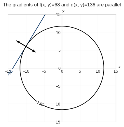
The gradients of \(f(x, y)\) and \(g(x, y)\) are \(\nabla f(x,y) = \begin{bmatrix}5\\-3\end{bmatrix}\) and \(\nabla g(x,y) = \begin{bmatrix}2x\\2y\end{bmatrix}\).

At the point \([-10, 6]\) the two gradients are \(\nabla f(-10,6) = \begin{bmatrix}5\\-3\end{bmatrix}\) and \(\nabla g(-10,6) = \begin{bmatrix}-20\\12\end{bmatrix}\).

The two vectors are parallel, so we can multiply one by some constant to get the other.

\(\begin{bmatrix}5\\-3\end{bmatrix} = -\cfrac{1}{4} \begin{bmatrix}-20\\12\end{bmatrix}\)

\(\nabla f(-10,6) = -\cfrac{1}{4} \nabla g(-10,6)\)

In general, we can conclude that a contour line of \(f(x, y)\) is tangent to a contour line of \(g(x, y)\) at the point \([x_0, y_0]\) if

\(\nabla f(x_0, y_0) = \lambda \nabla g(x_0, y_0)\)

In our example, this equivalence generates the following system of equations.

\(\begin{cases} 5 = \lambda 2x\\ -3 = \lambda 2y \end{cases}\)

At this point one might be tempted to solve it for \(x\), \(y\) and \(\lambda\), but the system is underdetermined because there are more unknowns than equations in the system.

Moreover, the system only helps us find a contour of \(f(x, y)\) that is tangent to a contour of \(g(x, y)\).

However, we are not interested in just any contour. We want it to be tangent to the contour \(g(x, y) = 136\).

The system we need to solve is

\(\begin{cases} 5 = \lambda 2x\\ -3 = \lambda 2y\\ x^2 + y^2 = 136\\ \end{cases}\)

Let’s practice solving system of equations manually.

\(\begin{cases} \cfrac{5}{\lambda 2} = x\\ -\cfrac{3}{2y} = \lambda\\ x^2 + y^2 = 136\\ \end{cases}\)

\(\begin{cases} \cfrac{5}{\lambda 2} = x\\ -\cfrac{3}{2y} = \lambda\\ \cfrac{25}{4\lambda^2} + y^2 = 136\\ \end{cases}\)

\(\begin{cases} \cfrac{5}{\lambda 2} = x\\ -\cfrac{3}{2y} = \lambda\\ \cfrac{25}{4} (-\cfrac{3}{2y})^{-2} + y^2 = 136\\ \end{cases}\)

\(\begin{cases} \cfrac{5}{\lambda 2} = x\\ -\cfrac{3}{2y} = \lambda\\ \cfrac{25}{4} 3^{-2} 4y^2 + y^2 = 136\\ \end{cases}\)

\(\begin{cases} \cfrac{5}{\lambda 2} = x\\ -\cfrac{3}{2y} = \lambda\\ \cfrac{25}{4} \cfrac{4y^2}{3^2} + y^2 = 136\\ \end{cases}\)

\(\begin{cases} \cfrac{5}{\lambda 2} = x\\ -\cfrac{3}{2y} = \lambda\\ \cfrac{25y^2}{3^2} + y^2 = 136\\ \end{cases}\)

\(\begin{cases} \cfrac{5}{\lambda 2} = x\\ -\cfrac{3}{2y} = \lambda\\ \cfrac{25y^2+ 9y^2}{9} = 136\\ \end{cases}\)

\(\begin{cases} \cfrac{5}{\lambda 2} = x\\ -\cfrac{3}{2y} = \lambda\\ \cfrac{34y^2}{9} = 136\\ \end{cases}\)

\(\begin{cases} \cfrac{5}{\lambda 2} = x\\ -\cfrac{3}{2y} = \lambda\\ 34y^2 = 1224\\ \end{cases}\)

\(\begin{cases} \cfrac{5}{\lambda 2} = x\\ -\cfrac{3}{2y} = \lambda\\ y^2 = 36\\ \end{cases}\)

\(\begin{cases} \cfrac{5}{\lambda 2} = x\\ -\cfrac{3}{2y} = \lambda\\ y = 6\\ y = -6\\ \end{cases}\)

Let’s solve for \(y = 6\)

\(\begin{cases} \cfrac{5}{\lambda 2} = x\\ -\cfrac{3}{2y} = \lambda\\ y = 6\\ \end{cases}\)

\(\begin{cases} \cfrac{5}{\lambda 2} = x\\ -\cfrac{3}{12} = \lambda\\ y = 6\\ \end{cases}\)

\(\begin{cases} \cfrac{5}{-\frac{2}{4}} = x\\ -\cfrac{1}{4} = \lambda\\ y = 6\\ \end{cases}\)

\(\begin{cases} x = -10\\ \lambda = -\cfrac{1}{4}\\ y = 6\\ \end{cases}\)

For \(y = -6\) we swap signs

\(\begin{cases} x = 10\\ \lambda = \cfrac{1}{4}\\ y = -6\\ \end{cases}\)

Let’s verify it.

x, y = sp.symbols("x, y")
f = 5 * x - 3 * y
g = x**2 + y**2
lam = sp.symbols("lambda")
solutions = sp.solve(
    [
        sp.diff(f, x) - lam * sp.diff(g, x),
        sp.diff(f, y) - lam * sp.diff(g, y),
        g - 136,
    ],
    [x, y, lam],
    dict=True,
)

for s in solutions:
    z = sp.lambdify((x, y), f, "numpy")(s[x], s[y])
    fig.add_scatter3d(
        x=[float(s[x])],
        y=[float(s[y])],
        z=[float(z)],
        showlegend=False,
        marker=dict(color="#67001F" if z > 0 else "#053061"),
        name="maximum" if z > 0 else "minimum",
    )
fig.update_layout(
    title="Maximum and minimum of the constrained problem",
)
fig.show()

We basically explained how the Lagrange multiplier method works, but at this point one might be wondering where the name comes from.

It turns out that the system can be expressed using the partial derivatives of the Lagrangian function

\(\mathcal{L}(x, y, \lambda) = f(x, y) - \lambda g(x, y)\)

😉 Although it doesn’t matter from a numerical perspective the Lagrangian is conventionally formed with a minus for maximization problems and a plus for minimization problems. It does matter if \(\lambda\) has an interpretation, like in economics.

Such system is shown below.

\(\begin{cases} \cfrac{\partial \mathcal{L}}{\partial x} = 0\\ \cfrac{\partial \mathcal{L}}{\partial y} = 0\\ \cfrac{\partial \mathcal{L}}{\partial \lambda} = 0 \end{cases}\)

Recall our problem is \(\min 5x - 3y \text{ s.t } x^2 + y^2 = 136\).

The Lagrangian for this problem is \(\mathcal{L}(x, y, \lambda) = 5x - 3y - \lambda(x^2 + y^2 - 136)\)

\(\begin{cases} \cfrac{\partial \mathcal{L}}{\partial x}5x - 3y - \lambda(x^2 + y^2 - 136) = 0\\ \cfrac{\partial \mathcal{L}}{\partial y}5x - 3y - \lambda(x^2 + y^2 - 136) = 0\\ \cfrac{\partial \mathcal{L}}{\partial \lambda}5x - 3y - \lambda(x^2 + y^2 - 136) = 0 \end{cases}\)

\(\begin{cases} 5 - \lambda 2x = 0\\ -3 - \lambda 2y = 0\\ x^2 + y^2 - 136 = 0 \end{cases}\)

Which is exactly the system we solved earlier.

\(\begin{cases} 5 = \lambda 2x\\ -3 = \lambda 2y\\ x^2 + y^2 = 136 \end{cases}\)

Convex optimization

🔑 Convex optimization entails the minimization of convex objective functions over a feasible convex sets. If the objective function and the constraints are both linear the problem is solved by linear programming. If the objective function is quadratic and the constraints are linear the problem is solved by quadratic programming.

Let \(\textbf{P}\) a convex optimization problem

\(\begin{array}{l} \textbf{P} \\ \min \limits_{x} f(x) \\ \text{subject to} \quad g_i(x) \ge 0 \quad \forall i=1,\dots,m \end{array}\)

where:

• \(f(x)\) is a convex function

• \(g_i(x)\) are linear functions defining a convex set

🔑 A function is convex if every point on the line segment connecting any two points \(a\) and \(b\) on the function lies completely above the function

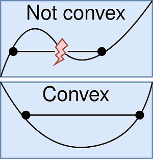Source: www.wikipedia.org

🔑 A set is convex if every point on the line segment connecting any two points \(a\) and \(b\) in the set lies completely within the set

Source: www.hacarus.com

Let’s take a look at the convex set created by the linear inequality constraint \(x \ge y\).

fig, ax = plt.subplots()
x_ = np.linspace(-30, 30)
y_ = x_
ax.plot(x_, y_, "tab:blue", lw=1)
ax.scatter(5, -5, color="tab:blue")
ax.text(3, -4.5, "5 - (-5) = 10", color="tab:blue")
ax.scatter(-5, 5, color="tab:orange")
ax.text(-6.5, 5.5, "-5 - 5 = -10", color="tab:orange")
ax.fill_between(x_, y_, -10, color="tab:blue", alpha=0.1)
ax.spines[["left", "bottom"]].set_position(("data", 0))
ax.text(1.02, 0, "$x$", transform=ax.get_yaxis_transform())
ax.text(0, 1.02, "$y$", transform=ax.get_xaxis_transform())
ax.set_xlim(-10, 10)
ax.set_ylim(-10, 10)
plt.title("The linear constraint $x - y \\geq 0$ defines a convex set", pad=20.0)
plt.show()

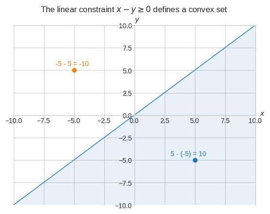
The point \((-5, 5)\) doesn’t satisfy the constraint because \(-5 < 5\), or alternatively \(-10 < 0\).

The point \((5, -5)\) does satisfy the constraint because \(5 \ge -5\) and so it does any point on and below the line \(y = x\).

Moreover, we can visually verify that the half space below the line is convex because every point on the line segment connecting any two points \(a\) and \(b\) in the set lies completely within the set.

🔑 Any linear constraint defines a convex set and a set of simultaneous linear constraints defines the intersection of convex sets, so it is also a convex set

Let’s take a look at the convex set resulting from the following \(g_i(x, y)\) inequality constraints

\(y - 1 \ge 0\)

\(x + 9 - y \ge 0\)

\(-\cfrac{3}{2}x + 9 - y \ge 0\)

\(\cfrac{1}{2}x + 6 - y \ge 0\)

\(-\cfrac{6}{5}x + 6 - y \ge 0\)

def fixup_animation_js(html_animation):
    html_animation = html_animation.replace(
        '<div class="anim-controls">',
        '<div class="anim-controls" style="display:none">',
    )
    animation_id = re.findall(r"onclick=\"(.*)\.", html_animation)[0]
    img_id = re.findall(r"<img id=\"(.*)\"", html_animation)[0]
    html_animation += f"""
<script language="javascript">
setupAnimationIntersectionObserver('{animation_id}', '{img_id}');
</script>
"""
    return html_animation


def _update(frame):
    global convex_set, half_space, in_set, out_set
    half_space.remove()
    convex_set.remove()
    in_set.remove()
    out_set.remove()
    ax.plot(x_, Y[:, frame], "tab:blue", lw=1)
    line = LineString(list(zip(x_, Y[:, frame])))
    poly = Polygon([line.coords[0], line.coords[-1], vertices[frame]])
    (half_space,) = ax.fill(*poly.exterior.xy, color="tab:blue", alpha=0.1)
    if frame > 0:
        poly_inter = poly.intersection(polygons[-1])
    else:
        poly_inter = poly
    polygons.append(poly_inter)
    (convex_set,) = ax.fill(*poly_inter.exterior.xy, color="tab:blue", alpha=0.5)
    in_set = ax.scatter(0, 1, color="tab:blue", marker="o", label="In set")
    ax.spines[["left", "bottom"]].set_position(("data", 0))
    out_set = ax.scatter(
        5 / 2,
        5,
        color="tab:blue" if frame < 4 else "tab:orange",
        marker="d",
        label="In set" if frame < 4 else "Not in set",
        zorder=2,
    )
    ax.legend(loc="upper right")


fig, ax = plt.subplots()
x_ = np.linspace(-30, 30, 250)
Y = np.zeros((250, 5))
Y[:, 0] = np.full_like(x_, 1)
m = np.array([1, -1.5, 0.5, -1.2])
b = np.array([9, 9, 6, 6])
Y[:, 1:] = m * x_.reshape(-1, 1) + b
vertices = [(-30, 30), (30, -30), (-30, -30), (30, -30), (-30, -30)]
polygons = []
(half_space,) = ax.fill([], [])
(convex_set,) = ax.fill([], [])
in_set = ax.scatter([], [])
out_set = ax.scatter([], [])
ax.spines[["left", "bottom"]].set_position(("data", 0))
ax.text(1.02, 0, "$x$", transform=ax.get_yaxis_transform())
ax.text(0, 1.02, "$y$", transform=ax.get_xaxis_transform())
ax.set_xlim(-10, 10)
ax.set_ylim(-5, 10)
plt.title(
    "Multiple linear constraints define the intersection of convex sets", pad=20.0
)

ani = FuncAnimation(fig, _update, frames=Y.shape[1], repeat=False, interval=1000)
html_animation = ani.to_jshtml(default_mode="loop")
if "runtime" not in get_ipython().config.IPKernelApp.connection_file:
    html_animation = fixup_animation_js(html_animation)
display(HTML(html_animation))
plt.close()

Once Loop Reflect

Let’s see if \((0, 1)\) belongs to the feasible set

\(0 \ge 0\)

\(8 \ge 0\)

\(8 \ge 0\)

\(5 \ge 0\)

\(5\ge 0\)

All constraints are satisfied.

What about \((\cfrac{5}{2}, 5)\)?

\(4 \ge 0\)

\(\cfrac{13}{2} \ge 0\)

\(\cfrac{1}{4} \ge 0\)

\(\cfrac{9}{4} \ge 0\)

\(-2 < 0\)

The last constraint is not satisfied.

Inequality constraints and the Karush–Kuhn–Tucker conditions

Let \(\textbf{P}\) a problem with \(m\) inequality constraints

\(\begin{array}{l} \textbf{P} \\ \min \limits_{x} f(x) \\ \text{subject to} \quad g_i(x) \ge 0 \quad \forall i=1,\dots,m \end{array}\)

It turns out inequality constraints can be formulated as equality constraints by introducing a non-negative slack variable \(s\).

\(\begin{array}{l} \min \limits_{x} f(x) \\ \text{subject to} \quad g_i(x) - s_i = 0 \end{array}\)

• If \(g_i(x)>0\): The slack variable \(s_i\) takes the value \(−g_i(x)\), so the sum is zero.

• If \(g_i(x)=0\): The slack variable \(s_i\) is zero.

• If \(g_i(x)<0\): No non-negative value of \(s_i\) can make the sum zero, which makes the equality unachievable, so it honours the original constraint.

The Lagrangian of this problem is

\(\mathcal{L}(x, \lambda, s) = f(x) - \sum \limits_{i=1}^{m} \lambda_i(g_i(x) - s_i)\)

This problem has an optimal solution only if the complementary slackness condition is met.

🔑 The complementary slackness condition states that at the optimal solution, either the Lagrange multipliers \(\lambda_i\) are zero or the respective constraints are active (the equality constraint \(g_i(x^{\star}) = 0\) holds).

The complementary slackness condition is expressed as \(\lambda_i g_i(x^{\star}) = 0\) \(\forall i=1,\dots,m\).

While it was useful to see the slack variable, in practice we do not add the slack variables but rather we “limit” the Lagrange multipliers for inequality constraints as non-negative.

\(\begin{array}{l} \textbf{P} \\ \min \limits_{x} f(x) \\ \text{subject to} \quad g_i(x) \ge 0 \quad \forall i=1,\dots,m \end{array}\)

The Lagrangian of \(\textbf{P}\) is simply as if \(g_i(x)\) were equality constraints.

\(\mathcal{L}(x, \lambda) = f(x) - \sum \limits_{i=1}^{m} \lambda_i g_i(x)\)

Note that we haven’t explicitly added any constraints for the Lagrange multipliers to be non-negative.

It’s just an additional condition for the problem to have an optimal solution, called dual feasibility.

🔑 The dual feasibility condition states that at the optimal solution, the Lagrange multipliers \(\lambda_i\) must be non-negative.

The dual feasibility condition is expressed as \(\lambda_i \ge 0\) \(\forall i=1,\dots,m\).

The complementary slackness and dual feasibility conditions are two of the four conditions known as Karush–Kuhn–Tucker (KKT) conditions.

The other two, stationarity and primal feasibility conditions simply state that at the optimal solution the gradient of the Lagrangian must be zero and all the constraints are satisfied.

As an example, let \(\textbf{Q}\) a convex optimization problem with a quadratic objective function and three linear inequality constraint defining a bounded convex set.

\(\begin{array}{l} \textbf{Q} \\ \min \limits_{x, y} x^2+y^2 \\ \text{subject to} \quad y + 4 \ge 0 \\ \quad \quad \quad \quad \quad x - y -\cfrac{3}{2} \ge 0 \\ \quad \quad \quad \quad \quad - \cfrac{3}{2}x - y + 9 \ge 0 \end{array}\)

Let’s build our intuition of this problem by looking at the contour plot.

x, y = sp.symbols("x, y")
f = x**2 + y**2

x_ = np.linspace(-30, 30, 250)
y_ = np.linspace(-30, 30, 250)
xx, yy = np.meshgrid(x_, y_)

fig, ax = plt.subplots()
cs = ax.contour(
    xx,
    yy,
    sp.lambdify((x, y), f, "numpy")(xx, yy),
    levels=np.floor(np.linspace(1, 50, 11)),
    cmap="RdBu_r",
)
polygons = []
Y = np.zeros((250, 3))
Y[:, 0] = np.full_like(x_, -4)
m = np.array([1, -1.5])
b = np.array([-1.5, 9])
Y[:, 1:] = m * x_.reshape(-1, 1) + b
vertices = [(-30, 30), (30, -30), (-30, -30)]
for i in range(Y.shape[1]):
    line = LineString(list(zip(x_, Y[:, i])))
    poly = Polygon([line.coords[0], line.coords[-1], vertices[i]])
    if i > 0:
        poly_inter = poly.intersection(polygons[-1])
    else:
        poly_inter = poly
    polygons.append(poly_inter)
ax.fill(
    *poly_inter.exterior.xy,
    color="tab:blue",
    alpha=0.5,
    edgecolor="k",
    linewidth=2,
    zorder=2
)

ax.clabel(cs, inline=True, fontsize=10)
ax.spines[["left", "bottom"]].set_position(("data", 0))
ax.text(1.02, 0, "$x$", transform=ax.get_yaxis_transform())
ax.text(0, 1.02, "$y$", transform=ax.get_xaxis_transform())
ax.set_xlim(-10, 10)
ax.set_ylim(-10, 10)
ax.set_aspect("equal")
plt.title("The problem $\\text{Q}$", pad=20.0)

Text(0.5, 1.0, 'The problem $\\text{Q}$')

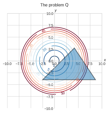
We can visually see that the minimum should be around \((0.75, -0.75)\) where one of the sides of the triangle is tangent to the \(f(x, y) = 1\) contour.

ax.scatter(
    0.75,
    -0.75,
    marker="*",
    color="tab:orange",
    s=100,
    edgecolors="k",
    linewidth=0.5,
    label="optimal solution",
    zorder=2,
)
ax.legend()
fig

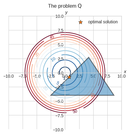
Let’s verify that \((0.75, -0.75)\) is indeed the optimal solution using the KKT conditions.

Before we do that we need to find the optimal values for \(\lambda_1\), \(\lambda_2\) and \(\lambda_3\).

Since \((0.75, -0.75)\) lies on the boundary of the second constraint, the second constraint is active. In fact,

\(\cfrac{3}{4} - (-\cfrac{3}{4}) -\cfrac{3}{2} = 0\)

As a consequence, the others constraints must be inactive. Thus, as per the complementary slackness condition, their respective Lagrange multiplies must be 0.

So for now we have that \(\lambda_1 = 0\) and \(\lambda_3 = 0\).

Let’s find \(\lambda_2\) by setting the partial derivatives of the Lagrangian to 0 and plugging in the optimal solution as well as \(\lambda_1 = 0\) and \(\lambda_3 = 0\).

The Lagrangian of \(\textbf{Q}\) is

\(\mathcal{L}(x, y, \lambda) = x^2 + y^2 - \lambda_{1} (y + 4) - \lambda_{2} (x - y - \cfrac{3}{2}) - \lambda_{3} (-\cfrac{3}{2} x - y + 9)\)

The partial derivatives wrt to \(x\) and \(y\) are

\(\cfrac{\partial\mathcal{L}}{\partial x} = 2x - \lambda_{2} + \cfrac{3}{2}\lambda_{3}\)

\(\cfrac{\partial\mathcal{L}}{\partial y} = 2y - \lambda_{1} + \lambda_{2} + \lambda_{3}\)

At the optimal solution and for \(\lambda_1 = 0\) and \(\lambda_3 = 0\)

\(\cfrac{\partial\mathcal{L}}{\partial x} = 0\)

\(2\cfrac{3}{4} - \lambda_{2} = 0\)

\(\lambda_{2} = \cfrac{3}{2}\)

\(\cfrac{\partial\mathcal{L}}{\partial y} = 0\)

\(-2\cfrac{3}{4} + \lambda_{2} = 0\)

\(\lambda_{2} = \cfrac{3}{2}\)

We can now verify that we’ve satisfied all the KKT conditions for this problem, which are shown below.

1. Stationarity

\(\nabla \mathcal{L}(x^{\star},y^{\star}) = 0\)

2. Primal feasibility

\(h_1(x^{\star},y^{\star}) \ge 0\)

\(h_2(x^{\star},y^{\star}) \ge 0\)

\(h_3(x^{\star},y^{\star}) \ge 0\)

3. Dual feasibility

\(\lambda_1^{\star} \ge 0\)

\(\lambda_2^{\star} \ge 0\)

\(\lambda_2^{\star} \ge 0\)

4. Complimentary slackness

\(\lambda_1^{\star}(h_1(x^{\star},y^{\star})) = 0\)

\(\lambda_2^{\star}(h_2(x^{\star},y^{\star})) = 0\)

\(\lambda_2^{\star}(h_3(x^{\star},y^{\star})) = 0\)

Let’s verify them all.

x, y = sp.symbols("x, y")
lam1, lam2, lam3 = sp.symbols("lambda_1, lambda_2, lambda_3", nonnegative=True)
f = x**2 + y**2
g1 = y + 4
g2 = x - y - sp.Rational(3, 2)
g3 = -sp.Rational(3, 2) * x - y + 9
lagrangian = f - lam1 * (g1) - lam2 * (g2) - lam3 * (g3)
dLx = sp.diff(lagrangian, x)
dLy = sp.diff(lagrangian, y)

sol = {x: 0.75, y: -0.75, lam1: 0, lam2: 1.5, lam3: 0}
# stationarity
assert dLx.subs(sol) == 0
assert dLy.subs(sol) == 0
# primal feasibility
assert g1.subs(sol) >= 0
assert g2.subs(sol) >= 0
assert g3.subs(sol) >= 0
# dual feasibility
assert sol[lam1] >= 0
assert sol[lam2] >= 0
assert sol[lam3] >= 0
# complementary slackness
assert sol[lam1] * g1.subs(sol) == 0
assert sol[lam2] * g2.subs(sol) == 0
assert sol[lam3] * g3.subs(sol) == 0

Let’s solve this problem analytically.

solutions = sp.solve(
    [dLx, dLy, lam1 * g1, lam2 * g2, lam3 * g3], [x, y, lam1, lam2, lam3], dict=True
)
valid_solutions = []
for sol in solutions:
    if g1.subs(sol) >= 0 and g2.subs(sol) >= 0 and g3.subs(sol) >= 0:
        valid_solutions.append(sol)

for sol in valid_solutions:
    for k, v in sol.items():
        display(Math(sp.latex(k) + "=" + sp.latex(v)))

$\displaystyle \lambda_{1}=0$

$\displaystyle \lambda_{2}=\frac{3}{2}$

$\displaystyle \lambda_{3}=0$

$\displaystyle x=\frac{3}{4}$

$\displaystyle y=- \frac{3}{4}$

Wolfe dual problem

🔑 The duality principle states that optimization problems may be viewed from either of two perspectives, the primal problem or the dual problem. If the primal is a minimization problem then the dual is a maximization problem (and vice versa).

As before, let \(\textbf{P}\) a convex optimization problem with \(m\) inequality constraints

\(\begin{array}{l} \textbf{P} \\ \min \limits_{x} f(x) \\ \text{subject to} \quad g_i(x) \ge 0 \quad \forall i=1,\dots,m \end{array}\)

This is the primal problem and the Lagrangian of \(\textbf{P}\) is the usual

\(\mathcal{L}(x, \lambda) = f(x) - \sum \limits_{i=1}^{m} \lambda_i g_i(x)\)

For a convex problem \(\textbf{P}\), its corresponding dual problem is termed as the Wolfe dual.

\(\begin{array}{l} \textbf{WD}_P \\ \max \limits_{\lambda} h(\lambda)\\ \text{subject to} \quad \lambda_i \ge 0 \quad \forall i=1,\dots,m \end{array}\)

where \(h(\lambda) = \min \limits_{x} \mathcal{L}(x, \lambda)\).

Recall the KKT conditions and note how the dual feasibility condition \(\lambda \ge 0\) refers to the satisfaction of the constraints of the dual problem, similarly to how the primal feasibility condition \(g(x) \ge 0\) refers to the constraints of the constraints of the primal problem.

\(h(\lambda)\) is the Lagrangian uniquely expressed as a linear function of \(\lambda\) evaluated at the optimal solution \(x^{\star}\).

It’s obtained by setting the partial derivative of the Lagrangian wrt x to 0, solving it for \(x^{\star}\) and substituting its equation back into the Lagrangian so \(x\) is removed.

This is best explained with an example.

Recall, the problem \(\textbf{Q}\)

\(\begin{array}{l} \textbf{Q} \\ \min \limits_{x, y} x^2+y^2 \\ \text{subject to} \quad y + 4 \ge 0 \\ \quad \quad \quad \quad \quad x - y -\cfrac{3}{2} \ge 0 \\ \quad \quad \quad \quad \quad - \cfrac{3}{2}x - y + 9 \ge 0 \end{array}\)

whose Lagrangian is

\(\mathcal{L}(x, y, \lambda) = x^2 + y^2 - \lambda_{1} (y + 4) - \lambda_{2} (x - y - \cfrac{3}{2}) - \lambda_{3} (-\cfrac{3}{2} x - y + 9)\)

To obtain \(h(\lambda) = \min \limits_{x} \mathcal{L}(x, \lambda)\) we set the partial derivatives of the Lagrangian to 0, solve for \(x^{\star}\) and \(y^{\star}\) and substitute their respective linear functions of \(\lambda\) back into the Lagrangian.

\(\cfrac{\partial\mathcal{L}}{\partial x} = 0\)

\(2x^{\star} - \lambda_{2} + \cfrac{3}{2}\lambda_{3} = 0\)

\(x^{\star} = \cfrac{2\lambda_{2}-3\lambda_{3}}{4}\)

\(\cfrac{\partial\mathcal{L}}{\partial y} = 0\)

\(2y - \lambda_{1} + \lambda_{2} + \lambda_{3} = 0\)

\(y^{\star} = \cfrac{\lambda_{1} - \lambda_{2} - \lambda_{3}}{2}\)

\(h(\lambda) = \cfrac{(2 \lambda_{2} - 3 \lambda_{3})^{2}}{16} + \cfrac{(\lambda_{1} - \lambda_{2} - \lambda_{3})^{2}}{4} - \lambda_{1} \left(\cfrac{\lambda_{1} - \lambda_{2} - \lambda_{3}}{2} + 4\right) - \lambda_{2} \left(\cfrac{2 \lambda_{2} - 3 \lambda_{3}}{4} - \cfrac{\lambda_{1} - \lambda_{2} - \lambda_{3}}{2} - \cfrac{3}{2}\right) - \lambda_{3} \left(- \cfrac{3 (2 \lambda_{2} - 3 \lambda_{3})}{8} - \cfrac{\lambda_{1} - \lambda_{2} - \lambda_{3}}{2} + 9\right)\)

The Wolfe dual problem can equivalently be formulated as

\(\begin{array}{l} \textbf{WD}_P \\ \max \limits_{x, \lambda} \mathcal{L}(x, \lambda)\\ \text{subject to} \quad \lambda_i \ge 0 \quad \forall i=1,\dots,m \\ \quad \quad \quad \quad \quad \cfrac{\partial}{\partial x}\mathcal{L}(x, \lambda) = 0 \end{array}\)

To analytically solve a minimization problem using the Lagrangian dual we can follow these steps:

1. Solve the Lagrangian dual for all \(\lambda_i\). We might need to solve it for different combinations of active constraints.

2. Evaluate the equations for \(x^{\star}\) and \(y^{\star}\) used to created \(h(\lambda)\)

3. Check the KKT conditions

x, y = sp.symbols("x, y")
lam1, lam2, lam3 = sp.symbols("lambda_1, lambda_2, lambda_3", nonnegative=True)
f = x**2 + y**2
g1 = y + 4
g2 = x - y - sp.Rational(3, 2)
g3 = -sp.Rational(3, 2) * x - y + 9
lagrangian = f - lam1 * (g1) - lam2 * (g2) - lam3 * (g3)
h = {
    x: sp.solve(sp.diff(lagrangian, x), x)[0],
    y: sp.solve(sp.diff(lagrangian, y), y)[0],
}
lagrangian_dual = lagrangian.subs(h)
eval_set = [
    dict(ChainMap(*t))
    for t in [
        c
        for i in range(1, 4)
        for c in combinations([{lam1: 0}, {lam2: 0}, {lam3: 0}], i)
    ]
]
valid_solutions = []
for e in eval_set:
    lambda_sol = sp.solve(
        [
            sp.diff(lagrangian_dual.subs(e), lam1),
            sp.diff(lagrangian_dual.subs(e), lam2),
            sp.diff(lagrangian_dual.subs(e), lam3),
        ],
        [lam1, lam2, lam3],
        dict=True,
    )
    if lambda_sol:
        for s in lambda_sol:
            x_star = h[x].subs(e | s)
            y_star = h[y].subs(e | s)
            sol = dict(ChainMap(e, s, {x: x_star, y: y_star}))
            assert (
                g1.subs(sol) >= 0 and g2.subs(sol) >= 0 and g3.subs(sol) >= 0
            ), "Primal feasibility not satisfied"
            assert (
                sol[lam1] * g1.subs(sol) == 0
                and sol[lam2] * g2.subs(sol) == 0
                and sol[lam3] * g3.subs(sol) == 0
            ), "Complementary slackness not satisfied"
            valid_solutions.append(sol)
for sol in valid_solutions:
    for k, v in sol.items():
        display(Math(sp.latex(k) + "=" + sp.latex(v)))

$\displaystyle x=\frac{3}{4}$

$\displaystyle y=- \frac{3}{4}$

$\displaystyle \lambda_{2}=\frac{3}{2}$

$\displaystyle \lambda_{3}=0$

$\displaystyle \lambda_{1}=0$

This might look like an unnecessary convoluted way to get to the same result we got by solving the primal problem directly, but the Lagrangian dual has become a common approach to solving optimization problems.

Many problems can be efficiently solved by constructing the Lagrangian function of the problem and solving the dual problem instead of the primal problem.

Optimizing SVM

Recall in Linear Algebra we applied concepts of linear algebra to SVM.

We derived the margin \(\gamma(w, b) = \min\cfrac{|wx_i+b|}{\|w\|}\) from the formula of the distance between a point a line \(d = \cfrac{|ax_0 + by_0 + b|}{\sqrt{a^2 + b^2}}\).

We then translated the objective in plain english “find the decision boundary that maximizes the margin between two classes such that the points belonging to each class lie on the correct side of the boundary” to the following constrained problem

\(\begin{array}{l} \min \limits_{w, b} \cfrac{1}{2} w \cdot w \\ \text{subject to } y_i(w \cdot x_i + b) \ge 1 \text{ } \forall i = 1, \dots, m \end{array}\)

We used scipy.minimize to solve it but we now have all the tools (Lagrange multipliers, KKT conditions, Wolfe dual) to solve it ourselves.

The Wolfe dual is

\(\begin{array}{l} \max \limits_{\alpha} h(\alpha)\\ \text{subject to} \quad \alpha_i \ge 0 \quad \forall i=1,\dots,m \end{array}\)

where \(h(\alpha) = \min \limits_{w, b} \mathcal{L}(w,b,\alpha)\).

Note we use \(\alpha\) instead of \(\lambda\) because it’s the notation commonly used in the SVM literature.

Let’s create the Lagrangian dual.

Step 1: Form the Lagrangian function of the primal

\(\mathcal{L}(w, b, \alpha) = \cfrac{1}{2} w \cdot w - \sum \limits_{i=1}^{m} \alpha_i[y_i(w \cdot x_i + b) - 1]\)

Step 2a: Calculate the partial derivative of \(\mathcal{L}(w, b, \alpha)\) wrt \(w\), set it to 0, solve for \(w^{\star}\) and substitute it into \(\mathcal{L}(w, b, \alpha)\) to obtain \(h(b, \alpha)\)

\(\cfrac{\partial}{\partial w}\mathcal{L} = 0\)

\(w^{\star} - \sum \limits_{i=1}^{m} \alpha_iy_ix_i = 0\)

\(w^{\star} = \left(\sum \limits_{i=1}^{m} \alpha_iy_ix_i\right)\)

\(h(b, \alpha) = \cfrac{1}{2} \left(\sum \limits_{i=1}^{m} \alpha_iy_ix_i\right) \cdot \left(\sum \limits_{j=1}^{m} \alpha_jy_jx_j\right) - \sum \limits_{i=1}^{m} \alpha_i[y_i(\left(\sum \limits_{j=1}^{m} \alpha_jy_jx_j\right) \cdot x_i + b) - 1]\)

\(= \cfrac{1}{2} \sum \limits_{i=1}^{m} \sum \limits_{j=1}^{m} \alpha_i\alpha_jy_iy_jx_i \cdot x_j - \sum \limits_{i=1}^{m} \sum \limits_{j=1}^{m} \alpha_i\alpha_jy_iy_jx_i \cdot x_j - b \sum \limits_{i=1}^{m} \alpha_iy_i + \sum \limits_{i=1}^{m} \alpha_i\)

\(= - \cfrac{1}{2} \sum \limits_{i=1}^{m} \sum \limits_{j=1}^{m} \alpha_i\alpha_jy_iy_jx_i \cdot x_j - b \sum \limits_{i=1}^{m} \alpha_iy_i + \sum \limits_{i=1}^{m} \alpha_i\)

Step 2b: Calculate the partial derivative of \(\mathcal{L}(w, b, \alpha)\) wrt \(b\), set it to 0, solve for \(b^{\star}\) and substitute it into \(\mathcal{L}(w, b, \alpha)\) to obtain \(h(\alpha)\)

\(\cfrac{\partial}{\partial b}\mathcal{L} = 0\)

\(-\sum \limits_{i=1}^{m} \alpha_iy_i = 0\)

To impose the partial derivative wrt to \(b\) to be 0 we’ll add a constraint to the dual problem.

\(\begin{array}{l} \max \limits_{\alpha} h(\alpha) \\ \text{subject to} \quad \alpha_i \ge 0 \quad \forall i=1,\dots,m \\ \quad \quad \quad \quad \quad \sum \limits_{i=1}^{m} \alpha_iy_i = 0 \end{array}\)

So we get that \(h(\alpha)\) is

\(h(\alpha) = - \cfrac{1}{2} \sum \limits_{i=1}^{m} \sum \limits_{j=1}^{m} \alpha_i\alpha_jy_iy_jx_i \cdot x_j - b\underbrace{\sum \limits_{i=1}^{m} \alpha_iy_i}_{0} + \sum \limits_{i=1}^{m} \alpha_i\)

\(= - \cfrac{1}{2} \sum \limits_{i=1}^{m} \sum \limits_{j=1}^{m} \alpha_i\alpha_jy_iy_jx_i \cdot x_j + \sum \limits_{i=1}^{m} \alpha_i\)

And here’s the dual we need to solve.

\(\begin{array}{l} \max \limits_{\alpha} \sum \limits_{i=1}^{m} \alpha_i - \cfrac{1}{2} \sum \limits_{i=1}^{m} \sum \limits_{j=1}^{m} \alpha_i\alpha_jy_iy_jx_i \cdot x_j \\ \text{subject to} \quad \alpha_i \ge 0 \quad \forall i=1,\dots,m \\ \quad \quad \quad \quad \quad \sum \limits_{i=1}^{m} \alpha_iy_i = 0 \end{array}\)

Once we’ve solved the Lagrangian dual for the multipliers \(\alpha\)’s, we get \(w^{\star}\) from

\(w^{\star} = \sum \limits_{i=1}^{m} \alpha_iy_ix_i\)

To get \(b^{\star}\), though, the process is a little bit more complicated.

We can use the constraint \(y_i(w \cdot x_i + b) - 1 \ge 0 \quad \forall i=1,\dots,m\).

Recall for the complementary slackness condition the constraint is equal to 0 when is active, so that \(\alpha_i\) may be greater than 0.

\(y_i(w \cdot x_i^{SV} + b) - 1 = 0 \quad \forall i=1,\dots,s\)

Note we put a \(SV\) superscript on the \(x_i\)’s for which the constraint is active, and \(s\) is the number of active constraints.

\(x_i^{SV}\) are the support vectors which the algorithm takes its name from.

We replace \(w\) with \(w^{\star}\) and we solve for \(b^{\star}\).

\(\sum \limits_{i=1}^{s} y_i(w^{\star} \cdot x_i^{SV} + b^{\star}) - 1 = 0\)

We multiply both sides by \(y_i\).

\(y_i \left[\sum \limits_{i=1}^{s} y_i(w^{\star} \cdot x_i^{SV} + b^{\star}) - 1 \right] = 0y_i\)

\(\sum \limits_{i=1}^{s} \left[y_i^2(w^{\star} \cdot x_i^{SV} + b^{\star}) - y_i \right] = 0\)

Because \(y_i \in \{-1, 1\}\) then \(y_i^2 = 1\)

\(\sum \limits_{i=1}^{s} w^{\star} \cdot x_i^{SV} + \sum \limits_{i=1}^{s} b^{\star} - \sum \limits_{i=1}^{s} y_i = 0\)

\(\sum \limits_{i=1}^{s} b^{\star} = \sum \limits_{i=1}^{s} y_i - \sum \limits_{i=1}^{s} w^{\star} \cdot x_i^{SV}\)

\(b^{\star} = \cfrac{1}{s} \sum \limits_{i=1}^{s} (y_i - w^{\star} \cdot x_i^{SV})\)

Let’s try to solve a small problem analytically.

m = 6
k = 2
neg_centroid = [-1, -1]
pos_centroid = [1, 1]

rng = np.random.default_rng(1)
X = np.r_[
    rng.standard_normal((m // 2, k)) + neg_centroid,
    rng.standard_normal((m // 2, k)) + pos_centroid,
].T
Y = np.array([[-1.0] * (m // 2) + [1.0] * (m // 2)])

fig, ax = plt.subplots()
ax.scatter(X[0], X[1], c=np.where(Y.squeeze() == -1, "tab:orange", "tab:blue"))
for i in range(m):
    ax.text(*X[:, i] + 0.2, i + 1, color="tab:orange" if Y[0, i] == -1 else "tab:blue")
ax.set_aspect("equal")
ax.set_xlabel("$x_1$")
ax.set_ylabel("$x_2$")
ax.set_xlim(-5, 5)
ax.set_ylim(-5, 5)
plt.title("Classification data")
plt.show()

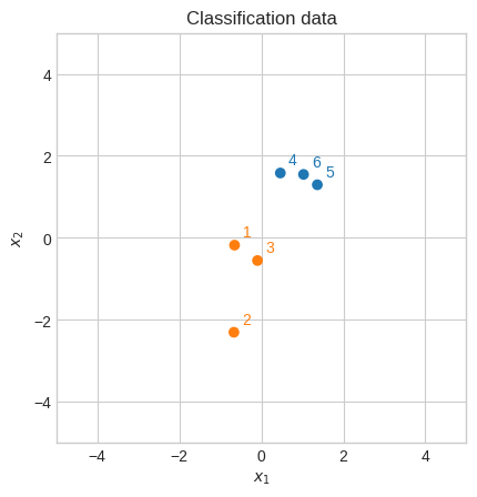
It seems that the support vectors are 1 and 4.

This helps us solve the Lagrangian dual analytically because we only need to solve it for \(\alpha_1\) and \(\alpha_2\). We’ll set the others to 0.

i = sp.symbols("i", cls=sp.Idx)
a = sp.IndexedBase("a", nonnegative=True)
x1 = sp.IndexedBase("x1")
x2 = sp.IndexedBase("x2")
y = sp.IndexedBase("y")
w1, w2, b = sp.symbols("w1, w2, b")
w = sp.Matrix([w1, w2])
x = sp.Matrix([x1[i], x2[i]])
f = (0.5 * w.T * w)[0]
g = y[i] * ((w.T * x)[0] + b) - 1
lagrangian = f - sp.Sum(a[i] * g, (i, 1, m))
dLw1 = sp.diff(lagrangian, w)[0]
dLw2 = sp.diff(lagrangian, w)[1]
dLb = sp.diff(lagrangian, b)
w1_star = sp.solve(dLw1, w1)[0]
w2_star = sp.solve(dLw2, w2)[0]
lagrangian_dual = (
    lagrangian.subs({w1: w1_star, w2: w2_star})
    .expand()
    .subs(sp.Sum(b * a[i] * y[i], (i, 1, m)), 0)
    .simplify()
)

display(Math("\\mathcal{h}(\\alpha) =" + sp.latex(lagrangian_dual)))

$\displaystyle \mathcal{h}(\alpha) =- 0.5 \left({a}_{1} {x_{1}}_{1} {y}_{1} + {a}_{2} {x_{1}}_{2} {y}_{2} + {a}_{3} {x_{1}}_{3} {y}_{3} + {a}_{4} {x_{1}}_{4} {y}_{4} + {a}_{5} {x_{1}}_{5} {y}_{5} + {a}_{6} {x_{1}}_{6} {y}_{6}\right)^{2} - 0.5 \left({a}_{1} {x_{2}}_{1} {y}_{1} + {a}_{2} {x_{2}}_{2} {y}_{2} + {a}_{3} {x_{2}}_{3} {y}_{3} + {a}_{4} {x_{2}}_{4} {y}_{4} + {a}_{5} {x_{2}}_{5} {y}_{5} + {a}_{6} {x_{2}}_{6} {y}_{6}\right)^{2} + {a}_{1} + {a}_{2} + {a}_{3} + {a}_{4} + {a}_{5} + {a}_{6}$

It turns out the system of equations resulting from the partial derivatives of \(h(\alpha)\) is quite complicated to be solved symbolically.

sympy conveniently features a numerical solver sympy.nsolve, although it’s not designed for it.

An alternative would be scipy.optimize.fsolve which can solve a system of non-linear equations.

We’ll stick with sympy for convenience, but later we’ll take a look at a low-level package specifically designed to solve quadratic programming problems called cvxopt.

sympy.nsolve requires an initial solution and we’ll also add verify=False to prevent above-tolerance errors.

We’ll use the KTT conditions to verify the solution ourselves.

data = dict(
    ChainMap(
        *[{x1[j + 1]: X[0, j], x2[j + 1]: X[1, j], y[j + 1]: Y[0, j]} for j in range(m)]
    )
)
a_fix = {a[2]: 0.0, a[3]: 0.0, a[5]: 0.0, a[6]: 0.0}

for a_0 in np.linspace(0.1, 1, 50):
    a_sol = sp.nsolve(
        [sp.diff(lagrangian_dual.subs(data | a_fix), a[j + 1]) for j in range(m)]
        + [sp.Sum(a[i] * y[i], (i, 1, m)).doit().subs(data | a_fix)],
        [a[1], a[4]],
        [a_0, a_0],
        dict=True,
        verify=False,
    )
    a_sol = a_fix | a_sol[0]
    if sp.Sum(a[i] * y[i], (i, 1, m)).doit().subs(data | a_sol) == 0:
        break

a_sol = {
    k: v
    for k, v in sorted(zip(a_sol.keys(), a_sol.values()), key=lambda a: a[0].indices)
}
for k, v in a_sol.items():
    display(Math(sp.latex(k) + "=" + str(v)))

$\displaystyle {a}_{1}=0.412244897959184$

$\displaystyle {a}_{2}=0.0$

$\displaystyle {a}_{3}=0.0$

$\displaystyle {a}_{4}=0.412244897959184$

$\displaystyle {a}_{5}=0.0$

$\displaystyle {a}_{6}=0.0$

Let’s verify the stationary condition for the dual.

for j in range(m):
    assert sp.diff(lagrangian_dual.subs(data | a_sol), a[j + 1]) == 0
assert sp.Sum(a[i] * y[i], (i, 1, m)).doit().subs(data | a_sol) == 0

Let’s calculate \(w^{\star}\) and \(b^{\star}\).

Recall

\(w^{\star} = \sum \limits_{i=1}^{m} \alpha_iy_ix_i\)

\(b^{\star} = \cfrac{1}{s} \sum \limits_{i=1}^{s} (y_i - w^{\star} \cdot x_i^{SV})\)

alpha = np.array(list(a_sol.values()), dtype="float")
sv = np.argwhere(alpha > 1e-5).squeeze()
w_star = (alpha * Y) @ X.T
b_star = np.mean(Y[:, sv] - w_star @ X[:, sv])

display(Math("w^{\\star} =" + sp.latex(sp.Matrix(w_star))))
display(Math("b^{\\star} =" + str(b_star)))

$\displaystyle w^{\star} =\left[\begin{matrix}0.460668244204358 & 0.725344881755978\end{matrix}\right]$

$\displaystyle b^{\star} =-0.4646549582754853$

It turns out we could have calculated \(w^{\star}\) just using the support vectors too, because the others \(\alpha_i\) are 0’s.

Although in practice the \(\alpha_i\) are never exactly 0. But in this case we can verify that it would have produced the exact same result.

assert np.array_equal(w_star, (alpha[sv] * Y[:, sv]) @ X[:, sv].T)

Let’s verify the KKT conditions for the primal.

wb_sol = {w1: w_star[0][0], w2: w_star[0][1], b: b_star}
sol = data | a_sol | wb_sol
# stationarity
assert dLw1.doit().subs(sol) == 0
assert dLw2.doit().subs(sol) == 0
assert dLb.doit().subs(sol) == 0
# primal feasibility
for j in range(m):
    try:
        g_eval = g.subs({i: j + 1}).subs(sol)
        assert g_eval >= 0, f"constraint {j+1} not satisfied: {g_eval:.2f}"
    except AssertionError as e:
        print(e)
# dual feasibility
for j in range(m):
    assert a_sol[a[j + 1]] >= 0
# complementary slackness
for j in range(m):
    try:
        ag_eval = a_sol[a[j + 1]] * g.subs({i: j + 1}).subs(sol)
        assert (
            ag_eval == 0
        ), f"complementary slackness {j+1} not satisfied: {ag_eval:.2f}"
    except AssertionError as e:
        print(e)

constraint 1 not satisfied: -0.10
constraint 3 not satisfied: -0.09
constraint 4 not satisfied: -0.10
complementary slackness 1 not satisfied: -0.04
complementary slackness 4 not satisfied: -0.04

We’re not at the optimal solution, but we’re close.

Let’s plot it.

plt.scatter(X[0], X[1], c=np.where(Y.squeeze() == -1, "tab:orange", "tab:blue"))
x1 = np.linspace(-4, 4, 100)
plt.plot(x1, (-w_star[0][0] * x1 - b_star) / w_star[0][1], color="k", alpha=0.5)
plt.scatter(
    X[0, sv],
    X[1, sv],
    s=80,
    facecolors="none",
    edgecolors="y",
    color="y",
    label="support vectors",
)
plt.xlabel("$x_1$")
plt.ylabel("$x_2$")
plt.title("Solution of the dual using sympy.nsolve")
plt.gca().set_aspect("equal")
plt.xlim(-5, 5)
plt.ylim(-5, 5)
plt.legend()
plt.show()

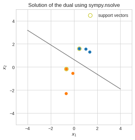
As mentioned earlier, sympy is not designed to solve this problem although in this case we managed to get an almost optimal solution.

We’ll now see how to solve this quadratic programming problem with the cvxopt library.

The cvxopt.solvers.qp function can solve the following primal quadratic programming problem

\(\begin{array}{l} \min \limits_{x} \cfrac{1}{2}x^TPx + q^Tx \\ \text{subject to} \quad Gx \preceq h \\ \quad \quad \quad \quad \quad Ax = b \end{array}\)

From the docstring of cvxopt.solvers.qp we see that it takes these parameters:

• \(P\): \((m \times m)\) d (double) cvxopt.matrix

• \(q\): \((m \times 1)\) d (double) cvxopt.matrix

• \(G\): \((m \times m)\) d (double) cvxopt.matrix

• \(h\): \((m \times 1)\) d (double) cvxopt.matrix

• \(A\): \((1 \times m)\) d (double) cvxopt.matrix

• \(b\): \((1 \times 1)\) d (double) cvxopt.matrix

The inequality constraints \(Gx \preceq h\) are

\(\begin{bmatrix} G_1&&0&&\dots&&0 \\ 0&&G_2&&\dots&&0 \\ \vdots&&\vdots&&\ddots&&\vdots \\ 0&&0&&\dots&&G_m \end{bmatrix} \begin{bmatrix} x_1 \\ x_2 \\ \vdots \\ x_m \\ \end{bmatrix} \preceq \begin{bmatrix} h_1 \\ h_2 \\ \vdots \\ h_m \\ \end{bmatrix} \Longrightarrow \begin{bmatrix} G_1x_1 \\ G_2x_2 \\ \vdots \\ G_mx_m \\ \end{bmatrix} \preceq \begin{bmatrix} h_1 \\ h_2 \\ \vdots \\ h_m \\ \end{bmatrix}\)

Note \(\preceq\) represent element-wise inequalities between two column vectors, in this case \(Gx\) which is \((m \times 1)\) and \(h\) which is also \((m \times 1)\).

The equality constraints \(Ax = b\) are

\(\begin{bmatrix} A_1&&A_2 \dots A_m \end{bmatrix} \begin{bmatrix} x_1 \\ x_2 \\ \vdots \\ x_m \\ \end{bmatrix}= \begin{bmatrix} b \end{bmatrix} \Longrightarrow A_1x_1 + A_2x_2 + \dots + A_mx_m= b\)

We need to re-write our problem so it conforms with cvxopt.solvers.qp requirements.

Recall the dual is

\(\begin{array}{l} \max \limits_{\alpha} \sum \limits_{i=1}^{m} \alpha_i - \cfrac{1}{2} \sum \limits_{i=1}^{m} \sum \limits_{j=1}^{m} \alpha_i\alpha_jy_iy_jx_i \cdot x_j \\ \text{subject to} \quad \alpha_i \ge 0 \quad \forall i=1,\dots,m \\ \quad \quad \quad \quad \quad \sum \limits_{i=1}^{m} \alpha_iy_i = 0 \end{array}\)

Writing as a minimization and with matrix notations becomes

\(\begin{array}{l} \min \limits_{\alpha} \cfrac{1}{2} \alpha^T (yy^Tx_i \cdot x_j) \alpha - \alpha \\ \text{subject to} \quad \alpha \succeq 0 \\ \quad \quad \quad \quad \quad y \alpha = 0 \end{array}\)

Then we note that: - \(x\) is \(\alpha\) (what cvxopt.solvers.qp solve for) and it’s a column vector - \(P\) corresponds to \((yy^Tx_i \cdot x_j)\) - \(q\) corresponds to a column vector of -1’s to make our minus a plus (\(q\) gets transposed) - \(G\) is a diagonal matrix of -1’s to make our \(\succeq\) a \(\preceq\) - \(h\) corresponds to a column vector of 0’s - \(A\) corresponds \(y\) which is a row vector - \(b\) corresponds to 0

Let \(P = yy^TK\), where \(K = x_i \cdot x_j\).

Let \(yy^T\) a square matrix resulting from the outer product of \(y\)

\(yy^T = \begin{bmatrix} y_1y_1&&\dots&&y_my_1\\ \vdots&&\ddots&&\vdots\\ y_my_1&&\dots&&y_my_m \end{bmatrix}\)

\(K = \begin{bmatrix} x_1 \cdot x_1&&\dots&&x_m \cdot x_1\\ \vdots&&\ddots&&\vdots\\ x_m \cdot x_1&&\dots&&x_m \cdot x_m \end{bmatrix}\)

K = np.array([np.dot(X[:, i], X[:, j]) for j in range(m) for i in range(m)]).reshape(
    (m, m)
)
P_mat = cvxopt.matrix(np.outer(Y, Y.T) * K)
assert P_mat.size == (m, m)
assert P_mat.typecode == "d"

Q_mat = cvxopt.matrix(np.full(m, -1.0))
assert Q_mat.size == (m, 1)
assert Q_mat.typecode == "d"

G_mat = cvxopt.matrix(np.diag(np.full(m, -1.0)))
assert G_mat.size == (m, m)
assert G_mat.typecode == "d"

h_mat = cvxopt.matrix(np.zeros(m))
assert h_mat.size == (m, 1)
assert h_mat.typecode == "d"

A_mat = cvxopt.matrix(Y, (1, m))
assert A_mat.size == (1, m)
assert A_mat.typecode == "d"

b_mat = cvxopt.matrix(0.0)
assert b_mat.size == (1, 1)
assert b_mat.typecode == "d"

solution = cvxopt.solvers.qp(
    P_mat, Q_mat, G_mat, h_mat, A_mat, b_mat, options=dict(show_progress=False)
)
alpha = np.ravel(solution["x"])
sv = np.argwhere(alpha > 1e-5).squeeze()
print(f"The support vectors are {sv+1}")

The support vectors are [1 4]

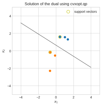
It seems our assumption about the support vectors earlier was indeed correct.

w_star = (alpha * Y) @ X.T
b_star = np.mean(Y[:, sv] - w_star @ X[:, sv])

display(Math("w^{\\star} =" + sp.latex(sp.Matrix(w_star))))
display(Math("b^{\\star} =" + str(b_star)))

$\displaystyle w^{\star} =\left[\begin{matrix}0.514414543271142 & 0.809980717346117\end{matrix}\right]$

$\displaystyle b^{\star} =-0.5188731465771707$

Let’s verify the KKT conditions.

a_sol = {a[j + 1]: a_val for j, a_val in enumerate(alpha)}
wb_sol = {w1: w_star[0][0], w2: w_star[0][1], b: b_star}
sol = data | a_sol | wb_sol
# stationarity
assert np.isclose(float(dLw1.doit().subs(sol)), 0, atol=1e-6)
assert np.isclose(float(dLw2.doit().subs(sol)), 0, atol=1e-6)
assert np.isclose(float(dLb.doit().subs(sol)), 0, atol=1e-6)
# primal feasibility
for j in range(m):
    try:
        g_eval = g.subs({i: j + 1}).subs(sol)
        assert g_eval >= 0, f"constraint {j} not satisfied: {g_eval:.2f}"
    except AssertionError as e:
        print(e)
# dual feasibility
for j in range(m):
    assert a_sol[a[j + 1]] >= 0
# complementary slackness
for j in range(m):
    try:
        ag_eval = float(a_sol[a[j + 1]] * g.subs({i: j + 1}).subs(sol))
        assert np.isclose(
            ag_eval, 0, atol=1e-6
        ), f"complementary slackness {j} not satisfied: {ag_eval:.2f}"
    except AssertionError as e:
        print(e)

This time they are all satisfied.

Let’s plot it again.

plt.scatter(X[0], X[1], c=np.where(Y.squeeze() == -1, "tab:orange", "tab:blue"))
x1 = np.linspace(-4, 4, 100)
plt.plot(x1, (-w_star[0][0] * x1 - b_star) / w_star[0][1], color="k", alpha=0.5)
plt.scatter(
    X[0, sv],
    X[1, sv],
    s=80,
    facecolors="none",
    edgecolors="y",
    color="y",
    label="support vectors",
)
plt.xlabel("$x_1$")
plt.ylabel("$x_2$")
plt.title("Solution of the dual using cvxopt.qp")
plt.gca().set_aspect("equal")
plt.xlim(-5, 5)
plt.ylim(-5, 5)
plt.legend()
plt.show()

Quasi-newton methods

While Newton’s method is a second-order optimization algorithm, Quasi-newton methods are a family of first-order optimization algorithms. The BFGS (Broyden–Fletcher–Goldfarb–Shanno) algorithm is one of the most popular.

One of the weaknesses of Newton’s method is its cost complexity.

🔑 Newton’s method has a cost complexity \(O(n^3)\); specifically, \(O(n^2)\) to calculate the Hessian, \(O(n^3)\) to calculate it and invert it.

Quasi-newton methods address exactly this issue.

🔑 Quasi-newton methods calculate an approximation of the Hessian at each step.

Quasi-newton optimization methods are a generalization of the secant method to find the root of the first derivative for multidimensional problems.

The secant method looks a lot like Newton’s method, but instead of one starting point, we have two starting points and the next point is the root of the secant joining these two points.

def secant(f, x, x0, x1):
    return f(x0) + ((f(x1) - f(x0)) / (x1 - x0)) * (x - x0)


def _update(frame):
    global x0_scat, x1_scat, x2_scat, min_scat, secant_line
    x0_scat.remove()
    x1_scat.remove()
    x2_scat.remove()
    secant_line.remove()
    min_scat.remove()
    x0_scat = ax.scatter(xs[frame - 1], df(xs[frame - 1]), color="tab:orange")
    x1_scat = ax.scatter(xs[frame], df(xs[frame]), color="tab:orange")
    (secant_line,) = ax.plot(
        xx,
        secant(df, xx, xs[frame - 1], xs[frame]),
        linestyle="--",
        color="tab:orange",
        label="secant",
    )
    x2_scat = ax.scatter(xs[frame + 1], 0, color="k", zorder=3)
    min_scat = ax.scatter(xs[frame + 1], f(xs[frame + 1]), color="tab:blue")


x = sp.symbols("x")
f = sp.exp(x) - sp.log(x)
df = sp.lambdify(x, sp.diff(f, x, 1))
f = sp.lambdify(x, f)

xs = [1.75, 0.25]
for _ in range(4):
    xs.append(xs[-1] - df(xs[-1]) * (xs[-1] - xs[-2]) / (df(xs[-1]) - df(xs[-2])))

fig, ax = plt.subplots()
xx = np.linspace(1e-3, 2)
ax.plot(xx, f(xx), color="tab:blue", label="$f(x)$")
ax.plot(xx, df(xx), color="tab:orange", label="$f'(x)$")
x0_scat = ax.scatter([], [])
x1_scat = ax.scatter([], [])
(secant_line,) = ax.plot([], [], linestyle="--", color="tab:orange", label="secant")
x2_scat = ax.scatter([], [])
min_scat = ax.scatter([], [])
ax.set_ylim(-5, 11)
ax.set_xlim(0, 2)
ax.spines[["left", "bottom"]].set_position(("data", 0))
ax.text(1, 0, "$x$", transform=ax.get_yaxis_transform())
ax.text(0, 1.02, "$f(x)$", transform=ax.get_xaxis_transform())
plt.legend(loc="upper right")
plt.title("Minimazation of $f(x)$ using the secant method")

ani = FuncAnimation(fig=fig, func=_update, frames=range(1, 5), interval=1000)
html_animation = ani.to_jshtml(default_mode="loop")
if "runtime" not in get_ipython().config.IPKernelApp.connection_file:
    html_animation = fixup_animation_js(html_animation)
display(HTML(html_animation))
plt.close()

Once Loop Reflect

Given two points \(\left(x_0, f(x_0)\right)\) and \(\left(x_1, f(x_1)\right)\), the slope of the line passing through these two points is the usual rise over run.

\(m = \cfrac{f(x_1) - f(x_0)}{x_1 - x_0}\)

Recall the point-slope form of a line \(y - y_1 = m(x - x_1)\).

So the line passing through \(\left(x_1, f(x_1)\right)\) is

\(y - f(x_1) = m(x - x_1)\)

Note we could have used \(\left(x_0, f(x_0)\right)\) too, but it would make the parallelism in notation with Newton’s method less obvious.

Replace \(m\) with the slope of the line passing through \(\left(x_0, f(x_0)\right)\) and \(\left(x_1, f(x_1)\right)\) and we get the equation of the secant line.

📐 \(y = \cfrac{f(x_1) - f(x_0)}{x_1 - x_0}(x - x_1)+f(x_1)\)

The root of this line is at

\(\cfrac{f(x_1) - f(x_0)}{x_1 - x_0}(x - x_1)+f(x_1) = 0\)

\(x = x_1 - f(x_1)\cfrac{x_1 - x_0}{f(x_1) - f(x_0)}\)

The general update formula of the secant optimization method is

\(x_{k+1} = x_{k} - f'(x_k)\cfrac{x_k - x_{k-1}}{f'(x_k) - f'(x_{k-1})}\)

Recall, the update of Newton’s method is

\(x_{k+1} = x_k - f'(x_k)\cfrac{1}{f''(x_k)}\)

If the two methods are indeed similar, it must follow that

\(\cfrac{x_k - x_{k-1}}{f'(x_k) - f'(x_{k-1})} \approx \cfrac{1}{f''(x_k)}\)

🔑 The secant method is an approximation of Newton’s method, for the same reason a secant line is an approximation of a tangent line

Recall in Week 1 we introduced derivatives by first talking about the average rate of change of function over interval \(\Delta x\) and then showing that as \(\Delta x\) approaches 0 we get to the instantaneous rate of change of the function, that is the derivative.

\(f'(x) = \lim_{{\Delta x}\to{0}}\cfrac{f(x + \Delta x) - f(x)}{\Delta x}\)

Let \(\Delta x = x_k - x_{k-1}\), and also \(x_{k-1} = x_k - \Delta x\) and we get

\(\lim_{{\Delta x}\to{0}} \cfrac{\Delta x}{f'(x_k) - f'(x_k - \Delta x)} = \cfrac{1}{f''(x_k)}\)

\(\lim_{{\Delta x}\to{0}} \cfrac{f'(x_k) - f'(x_k - \Delta x)}{\Delta x} = f''(x_k)\)

🔑 The rate of change of the first derivative over two consecutive steps of the secant method approximates the second derivative of Newton’s method

Although this relationship holds in the univariate case, things get more complicated with more variables.

Recall the update of Newton’s method in the multivariate case

\(p_{k+1} = p_k - H_f^{-1}(p_k) \cdot \nabla_f(p_k)\)

Let’s rewrite \(\lim_{{\Delta x}\to{0}} \cfrac{f'(x_k) - f'(x_k - \Delta x)}{\Delta x} = f''(x_k)\) as an approximation and we get

\(\cfrac{f'(x_k) - f'(x_k - \Delta x)}{\Delta x} \approx f''(x_k)\)

Let’s swap in the matrix notation and we get

\(\cfrac{\nabla_f(p_k) - \nabla f(p_k - \Delta p)}{\Delta p} \approx H_f(p_k)\)

\(\nabla_f(p_k) - \nabla f(p_k - \Delta p) \approx H_f(p_k) \Delta p\)

Earlier we let \(\Delta x = x_k - x_{k-1}\), so we can expand the notation to

\(\nabla_f(p_k) - \nabla f(p_k - p_k - p_{k-1}) \approx H_f(p_k)(p_k - p_{k-1})\)

\(\nabla_f(p_k) - \nabla_f(p_{k-1}) \approx H_f(p_k)(p_k - p_{k-1})\)

For the sake of consistency with the BFGS notation and conventions that we’ll introduce later, let’s increase the indices by 1 (our focus is determining the approximation of the Hessian for the \(k+1\) step), and let

\(y_k = \nabla_f(p_{k+1}) - \nabla_f(p_k)\)

\(s_k = p_{k+1} - p_k\)

\(H_{k+1} = H_f(p_{k+1})\)

So we get

\(y_k \approx H_{k+1}s_k\)

🔑 Quasi-newton methods finds an approximation \(B_{k+1}\) of \(H_{k+1}\) such that the condition \(y_k = B_{k+1}s_k\) (secant equation) is satisfied

It turns out we cannot solve \(y_k = B_{k+1}s_k\) for \(B_{k+1}\) because the system is underdetermined (more unknowns than equations in the system).

An underdetermined system can be solved by adding more equations, that is constraints.

The various Quasi-newton methods differ in terms of the constraints they specify.

BFGS

The BFGS algorithm solves the following constrained optimization problem at each update

\(\begin{array}{l} \textbf{P}_{BFGS} \\ \min \limits_{B_{k+1}} \|B_{k+1} - B_{k}\|_F \\ \text{subject to} \quad B_{k+1}^T = B_{k+1} \\ \quad \quad \quad \quad \quad y_k = B_{k+1}s_k \end{array}\)

In plain english, the BFGS algorithm minimizes the Frobenius norm (the equivalent of the Euclidean vector norm for a matrix) of the Hessian approximation between two consecutive updates such that the matrix is symmetric and the secant equation is satisfied.

Note that \(B_{k+1}^T = B_{k+1}\) is the symmetry constraint because a matrix is symmetric if it’s equal to its transpose.

sym_mat = np.array([[10, 2, 3], [2, 20, 3], [3, 3, 30]])
display(
    Math(
        "A_{sym} :="
        + sp.latex(sp.Matrix(sym_mat))
        + "="
        + sp.latex(sp.Matrix(sym_mat).T)
    )
)
assert np.array_equal(sym_mat, sym_mat.T)
not_sym_mat = np.array([[10, 3, 2], [2, 20, 3], [3, 3, 30]])
display(
    Math(
        "A_{nonsym} :="
        + sp.latex(sp.Matrix(not_sym_mat))
        + "\\neq"
        + sp.latex(sp.Matrix(not_sym_mat).T)
    )
)
assert not np.array_equal(not_sym_mat, not_sym_mat.T)

$\displaystyle A_{sym} :=\left[\begin{matrix}10 & 2 & 3\\2 & 20 & 3\\3 & 3 & 30\end{matrix}\right]=\left[\begin{matrix}10 & 2 & 3\\2 & 20 & 3\\3 & 3 & 30\end{matrix}\right]$

$\displaystyle A_{nonsym} :=\left[\begin{matrix}10 & 3 & 2\\2 & 20 & 3\\3 & 3 & 30\end{matrix}\right]\neq\left[\begin{matrix}10 & 2 & 3\\3 & 20 & 3\\2 & 3 & 30\end{matrix}\right]$

It turns out that the solution to \(\textbf{P}_{BFGS}\) ends up being equivalent to

\(\arg \min \limits_{B_{k+1}} \textbf{P}_{BFGS} = B_{k} + U_{k} + V_{k}\)

Let \(U_{k} = \alpha uu^T\) and \(V_{k} = \beta vv^T\), where:

• \(u\) and \(v\) are two linearly independent \((n \times 1)\) vectors, where \(n\) is the number of parameters of \(f(x_1, \dots, x_n)\)

• \(\alpha\) and \(\beta\) are two scalar

So we get

\(\arg \min \limits_{B_{k+1}} \textbf{P}_{BFGS} = B_{k} + \alpha uu^T + \beta vv^T\)

The outer products \(uu^T\) and \(vv^T\) mean that \(U\) and \(V\) are rank-one symmetric \((n \times n)\) matrices and the sum \(U_k + V_k\) is rank-two.

From Linear Algebra - Week 1 recall, that the rank of a matrix is the number of linearly independent rows.

For example, \(uu^T\) yields a matrix where \(n-1\) rows are linearly dependent because each row is a linear combination of \(u\).

These properties of \(U\) and \(V\) is what makes them part of the solution to \(\textbf{P}_{BFGS}\).

But perhaps, most importantly, need to find \(\alpha\), \(\beta\), \(u\) and \(v\) such that the solution satisfies the secant equation condition \(y_k = B_{k+1}s_k\).

Let’s impose the secant equation condition by multiplying each side by \(s_k\)

\(\underbrace{B_{k+1}s_k}_{y_k} = B_ks_k + \alpha uu^Ts_k + \beta vv^Ts_k\)

Let \(u = y_k\) and \(v = B_ks_k\) and we obtain

\(y_k = B_ks_k + \alpha y_ky_k^Ts_k + \beta B_ks_ks_k^TB_k^Ts_k\)

Note that, in general, the transpose of \(XY\) is \(Y^TX^T\), so the transpose of \(B_ks_k\) is \(s_k^TB_k^T\) but \(B_k^T=B_k\) by imposition of our problem, so we get

\(y_k - \alpha y_ky_k^Ts_k = B_ks_k + \beta B_ks_ks_k^TB_ks_k\)

\(y_k(1 - \alpha y_k^Ts_k) = B_ks_k(1 + \beta s_k^TB_ks_k)\)

\(\begin{cases} y_k(1 - \alpha y_k^Ts_k) = B_{k}s_k(1 + \beta s_k^TB_ks_k)\\ 1 - \alpha y_k^Ts_k = 0 \\ 1 + \beta s_k^TB_ks_k = 0 \end{cases}\)

\(\begin{cases} y_k(1 - \alpha y_k^Ts_k) = B_{k}s_k(1 + \beta s_k^TB_k^Ts_k)\\ \alpha = \cfrac{1}{y_k^Ts_k} \\ \beta = -\cfrac{1}{s_k^TB_ks_k} \end{cases}\)

Let’s replace \(\alpha\) and \(\beta\) back in and we get

\(y_k = B_{k}s_k + \left(\cfrac{1}{y_k^Ts_k}\right) y_ky_k^Ts_k + \left(-\cfrac{1}{s_k^TB_ks_k}\right) B_ks_ks_k^TB_ks_k\)

\(y_k = B_{k} + \cfrac{y_ky_k^T }{y_k^Ts_k} -\cfrac{B_ks_ks_k^TB_k}{s_k^TB_ks_k}\)

So we get that

\(B_{k+1} = B_{k} + \cfrac{y_ky_k^T}{y_k^Ts_k} -\cfrac{B_ks_ks_k^TB_k}{s_k^TB_ks_k}\)

Now, at this point we could invert \(B_{k+1}\) and we would be done but it would be more efficient if we could calculate the inverse directly.

\(B_{k+1}\) is a sum of matrices so its inverse is can be seen as a Woodbury matrix identity.

\((B+UV^T)^{-1}=B^{-1}-\cfrac{B^{-1}UV^TB^{-1}}{I+V^TB^{-1}U}\)

or equivalently

\((B+UV^T)^{-1}=B^{-1}-B^{-1}U(I+V^TB^{-1}U)^{-1}V^TB^{-1}\)

After some algebra which is shown in Derivation of the direct inverse of the BFGS update we get

\(B^{-1}_{k+1} = \left(I - \cfrac{s_ky_k^T}{y_k^Ts_k} \right)B^{-1}_k \left(I - \cfrac{y_ks_k^T}{y_k^Ts_k} \right) + \cfrac{s_ks_k^T}{y_k^Ts_k}\)

Let’s verify we can calculate \(B^{-1}_{k+1}\) directly using some synthetic data for \(y_k\), \(s_k\) and \(B_k\).

y = np.array([1, 2, 3])
s = np.array([3, 4, 5])
B = np.array([[1, 2, 3], [2, 2, 3], [3, 3, 3]])

B1 = (
    B
    + np.outer(y, y.T) / np.dot(y.T, s)
    - np.outer(B @ s, s.T @ B) / np.dot(np.dot(s.T, B), s)
)
expected = np.linalg.inv(B1)
direct_inverse = (np.identity(3) - np.outer(s, y) / np.dot(y, s)) @ np.linalg.inv(B) @ (
    np.identity(3) - np.outer(y, s) / np.dot(y, s)
) + np.outer(s, s) / np.dot(y, s)
assert np.allclose(direct_inverse, expected)

Let’s use the BFGS algorithm on a small problem we’ve seen before.

def bivariate_bfgs_algo(f, symbols, initial, steps):
    x, y = symbols
    nabla = sp.Matrix([sp.diff(f, x), sp.diff(f, y)])
    nabla_eval = sp.lambdify((x, y), nabla, "numpy")
    p = np.zeros((steps, 2))
    g = np.zeros((steps, 2))
    b_inv = np.zeros((steps, 2, 2))
    step_vector = np.zeros((steps, 2))
    p[0] = initial
    g[0] = nabla_eval(*p[0]).squeeze()
    b_inv[0] = np.identity(2)
    step_vector[0] = b_inv[0] @ g[0]
    for i in range(1, steps):
        p[i] = p[i - 1] - step_vector[i - 1]
        g[i] = nabla_eval(*p[i]).squeeze()
        # calculate approximate inverse hessian
        s_k = p[i] - p[i - 1]
        y_k = g[i] - g[i - 1]
        i_mat = np.identity(2)
        out1 = np.outer(s_k, y_k)
        out2 = np.outer(y_k, s_k)
        out3 = np.outer(s_k, s_k)
        dot1 = np.dot(y_k, s_k)
        b_inv[i] = (i_mat - out1 / dot1) @ b_inv[i - 1] @ (
            i_mat - out2 / dot1
        ) + out3 / dot1
        step_vector[i] = b_inv[i] @ g[i]
        if np.linalg.norm(step_vector[i]) < 1e-4:
            break
    return p[: i + 1], g[: i + 1], b_inv[: i + 1], step_vector[: i + 1]


x, y = sp.symbols("x, y")
g = x**4 + 0.8 * y**4 + 4 * x**2 + 2 * y**2 - x * y - 0.2 * x**2 * y
p, _, _, _ = bivariate_bfgs_algo(g, symbols=(x, y), initial=np.array([4, 4]), steps=100)

display(
    Math(
        "\\arg \\min \\limits_{x,y}"
        + sp.latex(g)
        + "="
        + sp.latex(np.array2string(p[-1], precision=2, suppress_small=True))
    )
)

$\displaystyle \arg \min \limits_{x,y}x^{4} - 0.2 x^{2} y + 4 x^{2} - x y + 0.8 y^{4} + 2 y^{2}=\mathtt{\text{[0. 0.]}}$

Let’s re-train a logistic regression model (single-neuron with sigmoid activation) on this classification data that we used in Week 3.

m = 40
k = 2
neg_centroid = [-1, -1]
pos_centroid = [1, 1]

rng = np.random.default_rng(1)
X = np.r_[
    rng.standard_normal((m // 2, k)) + neg_centroid,
    rng.standard_normal((m // 2, k)) + pos_centroid,
].T
Y = np.array([[0] * (m // 2) + [1] * (m // 2)])

plt.scatter(X[0], X[1], c=np.where(Y.squeeze() == 0, "tab:orange", "tab:blue"))
plt.gca().set_aspect("equal")
plt.xlabel("$x_1$")
plt.ylabel("$x_2$")
plt.xlim(-5, 5)
plt.ylim(-5, 5)
plt.title("Classification data")
plt.show()

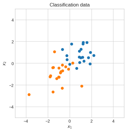
But this time we’ll use the BFGS algorithm instead of gradient descent.

def sigmoid(x):
    return 1 / (1 + np.exp(-x))


def init_neuron_params(k):
    w = rng.uniform(size=(1, k)) * 0.5
    b = np.zeros((1, 1))
    return {"w": w, "b": b}


def neuron_output(X, params, activation, *args):
    w = params["w"]
    b = params["b"]
    Z = w @ X + b
    Y_hat = activation(Z, *args)
    return Y_hat


def compute_log_loss(Y, Y_hat):
    m = Y_hat.shape[1]
    loss = (-1 / m) * (
        np.dot(Y, np.log(Y_hat).T) + np.dot((1 - Y), np.log(1 - Y_hat).T)
    )
    return loss.squeeze()


def compute_grads(X, Y, Y_hat):
    m = Y_hat.shape[1]
    dw = -1 / m * np.dot(Y - Y_hat, X.T)
    db = -1 / m * np.sum(Y - Y_hat, axis=1, keepdims=True)
    return np.hstack([dw.squeeze(), db.squeeze()])


def compute_approx_inverse_hessian(p_new, p_old, g_new, g_old, b_inv_old):
    s_k = p_new - p_old
    y_k = g_new - g_old
    i_mat = np.identity(b_inv_old.shape[0])
    out1 = np.outer(s_k, y_k)
    out2 = np.outer(y_k, s_k)
    out3 = np.outer(s_k, s_k)
    dot1 = np.dot(y_k, s_k)
    return (i_mat - out1 / dot1) @ b_inv_old @ (i_mat - out2 / dot1) + out3 / dot1


steps = 50

params = init_neuron_params(k)
Y_hat = neuron_output(X, params, sigmoid)
loss = compute_log_loss(Y, Y_hat)
print(f"Iter 0  - Log loss={loss:.6f}")

p = np.zeros((steps + 1, k + 1))
g = np.zeros((steps + 1, k + 1))
b_inv = np.zeros((steps + 1, k + 1, k + 1))
step_vector = np.zeros((steps + 1, k + 1))

p[0] = np.hstack([v.squeeze() for v in params.values()])
g[0] = compute_grads(X, Y, Y_hat)
b_inv[0] = np.identity(k + 1)
step_vector[0] = b_inv[0] @ g[0]

for i in range(1, steps + 1):
    p[i] = p[i - 1] - step_vector[i - 1]
    params = {"w": p[i][None, :k], "b": p[i][None, -1:]}
    Y_hat = neuron_output(X, params, sigmoid)
    loss_new = compute_log_loss(Y, Y_hat)
    if loss - loss_new <= 1e-4:
        print(f"Iter {i} - Log loss={loss:.6f}")
        print("The algorithm has converged")
        break
    loss = loss_new
    if i % 2 == 0:
        print(f"Iter {i} - Log loss={loss:.6f}")
    g[i] = compute_grads(X, Y, Y_hat)
    b_inv[i] = compute_approx_inverse_hessian(
        p_new=p[i], p_old=p[i - 1], g_new=g[i], g_old=g[i - 1], b_inv_old=b_inv[i - 1]
    )
    step_vector[i] = b_inv[i] @ g[i]

Iter 0  - Log loss=0.504431
Iter 2 - Log loss=0.228404
Iter 4 - Log loss=0.139608
Iter 6 - Log loss=0.106573
Iter 8 - Log loss=0.097015
Iter 10 - Log loss=0.096400
The algorithm has converged

Let’s compare it with the results obtained in Week 3 using gradient descent on the same data.

Iter 0  - Log loss=0.582076
Iter 100 - Log loss=0.182397
Iter 200 - Log loss=0.148754
Iter 300 - Log loss=0.134595
Iter 306 - Log loss=0.134088
The algorithm has converged

The results might be slightly different due to the random initialization.

Finally, let’s plot it.

w, b = params.values()
xx1, xx2 = np.meshgrid(np.linspace(-5, 5, 100), np.linspace(-5, 5, 100))

neg_scatter = go.Scatter3d(
    z=np.full(int(m / 2), 0),
    x=X[0, : int(m / 2)],
    y=X[1, : int(m / 2)],
    mode="markers",
    marker=dict(color="#ff7f0e", size=5),
    name="negative class",
)
pos_scatter = go.Scatter3d(
    z=np.full(int(m / 2), 1),
    x=X[0, int(m / 2) :],
    y=X[1, int(m / 2) :],
    mode="markers",
    marker=dict(color="#1f77b4", size=5),
    name="positive class",
)
final_model_plane = go.Surface(
    z=sigmoid(w[0, 0] * xx1 + w[0, 1] * xx2 + b),
    x=xx1,
    y=xx2,
    colorscale=[[0, "#ff7f0e"], [1, "#1f77b4"]],
    showscale=False,
    opacity=0.5,
    name="final params",
)

fig = go.Figure([pos_scatter, neg_scatter, final_model_plane])
fig.update_layout(
    title="Final model",
    autosize=False,
    width=600,
    height=600,
    margin=dict(l=10, r=10, b=10, t=30),
    scene=dict(
        xaxis=dict(title="x1", range=[-5, 5]),
        yaxis=dict(title="x2", range=[-5, 5]),
        zaxis_title="y",
        camera_eye=dict(x=0, y=0.3, z=2.5),
        camera_up=dict(x=0, y=np.sin(np.pi), z=0),
    ),
)

Derivation of the direct inverse of the BFGS update

The objective is to derive

\(B^{-1}_{k+1} = \left(I - \cfrac{s_ky_k^T}{y_k^Ts_k} \right)B^{-1}_k \left(I - \cfrac{y_ks_k^T}{y_k^Ts_k} \right) + \cfrac{s_ks_k^T}{y_k^Ts_k}\)

from

\(B^{-1}_{k+1} = \left(B_{k} + \cfrac{y_ky_k^T}{y_k^Ts_k} -\cfrac{B_ks_ks_k^TB_k}{s_k^TB_ks_k}\right)^{-1}\)

Using Woodbury matrix identity we get that the inverse of \(B_{k+1}\) is

\(B_{k+1}^{-1} = \left(\underbrace{B_{k} + \cfrac{y_ky_k^T}{y_k^Ts_k} -\cfrac{B_ks_ks_k^TB_k}{s_k^TB_ks_k}}_{(1)}\right)^{-1} = (B_k+UV^T)^{-1} = \underbrace{B_k^{-1}-B_k^{-1}U(I+V^TB_k^{-1}U)^{-1}V^TB_k^{-1}}_{(2)}\)

For the sake of a cleaner notation, let’s remove the \(k\) indexing from \((1)\).

\(B + \cfrac{yy^T}{y^Ts} -\cfrac{Bss^TB}{s^TBs}\)

It turns out the above expression can be rewritten as

\(\underbrace{B}_{n \times n}+ \underbrace{\begin{bmatrix}\overbrace{Bs}^{n \times 1}&&\overbrace{y}^{n \times 1}\end{bmatrix}}_{U \text{ } (n \times 2)} \underbrace{\overbrace{\begin{bmatrix}-\cfrac{1}{s^TBs}&&0\\0&&\cfrac{1}{y^Ts}\end{bmatrix}}^{V_1 \text{ } (2 \times 2)} \overbrace{\begin{bmatrix}s^TB\\y^T\end{bmatrix}}^{V_2 \text{ } (2 \times n)}}_{V^T \text{ } (2 \times n)}\)

To verify this and all the next operations we’ll be making, let’s create a simple example with \(n=3\).

y = np.array([1, 2, 3])
s = np.array([3, 4, 5])
B = np.array([[1, 2, 3], [2, 2, 3], [3, 3, 3]])
B1 = (
    B
    + np.outer(y, y.T) / np.dot(y.T, s)
    - np.outer(B @ s, s.T @ B) / np.dot(np.dot(s.T, B), s)
)

U = np.hstack([(B @ s)[:, None], y[:, None]])
V1 = np.array([[-1 / (s.T @ B @ s), 0], [0, 1 / (y.T @ s)]])
V2 = np.vstack([s.T @ B, y.T])
VT = V1 @ V2

print("Shapes:\n-------")
print("y: ", y.shape)
print("s: ", s.shape)
print("B: ", B.shape)
print("U: ", U.shape)
print("V1:", V1.shape)
print("V2:", V2.shape)
print("VT:", VT.shape)

Shapes:
-------
y:  (3,)
s:  (3,)
B:  (3, 3)
U:  (3, 2)
V1: (2, 2)
V2: (2, 3)
VT: (2, 3)

Finally, let’s verify that

\(B + \cfrac{yy^T}{y^Ts} -\cfrac{Bss^TB}{s^TBs} = B + UV^T\)

assert np.allclose(B1, B + U @ VT)

Let’s plug the substitutions for \(U\) and \(V^T\) into \((2)\) and we obtain

\(B^{-1}-B^{-1}\begin{bmatrix}Bs&&y\end{bmatrix} \left(I+\begin{bmatrix}-\cfrac{1}{s^TBs}&&0\\0&&\cfrac{1}{y^Ts}\end{bmatrix} \begin{bmatrix}s^TB\\y^T\end{bmatrix}B^{-1}\begin{bmatrix}Bs&&y\end{bmatrix}\right)^{-1}\begin{bmatrix}-\cfrac{1}{s^TBs}&&0\\0&&\cfrac{1}{y^Ts}\end{bmatrix}\begin{bmatrix}s^TB\\y^T\end{bmatrix}B^{-1}\)

Let’s verify that we can simplify \(B^{-1}U := B^{-1}\begin{bmatrix}Bs&&y\end{bmatrix}\) to \(\begin{bmatrix}s&&B^{-1}y\end{bmatrix}\) and let’s define it as \(D\).

D = np.hstack([s[:, None], (np.linalg.inv(B) @ y)[:, None]])
assert np.allclose(np.linalg.inv(B) @ U, D)
print("Shapes:\n-------")
print("D:", D.shape)

Shapes:
-------
D: (3, 2)

Let’s verify we can simplify \(V_2B^{-1} := \begin{bmatrix}s^TB\\y^T\end{bmatrix}B^{-1}\) to \(\begin{bmatrix}s^T\\y^TB^{-1}\end{bmatrix}\) and that is equivalent to \(D^T\), and so it follows that \(B^{-1}V_2^T = D\).

Note that \((B^{-1})^T\) is the same as \(B^{-1}\) because \(B\) is symmetric.

assert np.allclose(V2 @ np.linalg.inv(B), np.vstack([s.T, y.T @ np.linalg.inv(B)]))
assert np.allclose(D.T, np.vstack([s.T, y.T @ np.linalg.inv(B)]))
assert np.allclose(V2 @ np.linalg.inv(B), D.T)
assert np.allclose(np.linalg.inv(B) @ V2.T, D)

Let \(M\) the big bracketed expression in the middle.

\(B^{-1}-\underbrace{\begin{bmatrix}s&&B^{-1}y\end{bmatrix}}_{D \text{ } (n \times 2)} \underbrace{\left(\overbrace{I}^{(2 \times 2)}+ \overbrace{\begin{bmatrix}-\cfrac{1}{s^TBs}&&0\\0&&\cfrac{1}{y^Ts}\end{bmatrix}\begin{bmatrix}s^TB\\y^T\end{bmatrix}}^{2 \times n} \overbrace{B^{-1}}^{n \times n} \overbrace{\begin{bmatrix}Bs&&y\end{bmatrix}}^{(n \times 2)}\right)^{-1} \begin{bmatrix}-\cfrac{1}{s^TBs}&&0\\0&&\cfrac{1}{y^Ts}\end{bmatrix}}_{M^{-1} \text{ } (2 \times 2)} \underbrace{\begin{bmatrix}s^T\\y^TB^{-1}\end{bmatrix}}_{D^T \text{ } (2 \times n)}\)

M_inv = np.linalg.inv(np.identity(2) + VT @ np.linalg.inv(B) @ U) @ V1
print("Shapes:\n-------")
print("M_inv:", M_inv.shape)

Shapes:
-------
M_inv: (2, 2)

Let’s verify \(B^{-1}-DM^{-1}D^T\) is equivalent to \(\left(B_{k} + \cfrac{y_ky_k^T}{y_k^Ts_k} -\cfrac{B_ks_ks_k^TB_k}{s_k^TB_ks_k}\right)^{-1}\).

assert np.allclose(np.linalg.inv(B) - D @ M_inv @ D.T, np.linalg.inv(B1))

Let’s simplify \(M^{-1}\).

\(M^{-1} = (I + V^T B^{-1} U)^{-1} V_1\)

\(M^{-1} = [V_{1}^{-1} (I + V_1 V_2 B^{-1} U)]^{-1}\)

Earlier we simplified \(B^{-1} U\) to \(D\), so we get

\(M^{-1} = [V_{1}^{-1} (I + V_{1} V_{2} D)]^{-1}\)

\(M^{-1} = (V_{1}^{-1} + V_2 D)^{-1}\)

Let’s verify it.

assert np.allclose(M_inv, np.linalg.inv(np.linalg.inv(V1) + V2 @ np.linalg.inv(B) @ U))

So we have that \(M^{-1}\) is

\(M^{-1} = \left(\begin{bmatrix}-s^TBs&&0\\0&&y^Ts\end{bmatrix}+ \begin{bmatrix}s^TB\\y^T\end{bmatrix}B^{-1}\begin{bmatrix}Bs&&y\end{bmatrix}\right)^{-1}\)

It might not be obvious that the inverse of \(V1\) is \(\begin{bmatrix}-s^TBs&&0\\0&&y^Ts\end{bmatrix}\), so let’s verify it.

assert np.allclose(np.linalg.inv(V1), np.array([[-s.T @ B @ s, 0], [0, y.T @ s]]))

Let’s verify \(\begin{bmatrix}s^TB\\y^T\end{bmatrix}\begin{bmatrix}s&&B^{-1}y\end{bmatrix}\) becomes \(\begin{bmatrix}s^TBs&&s^Ty\\y^Ts&&y^TB^{-1}y\end{bmatrix}\).

assert np.allclose(
    V2 @ D, np.array([[s.T @ B @ s, s.T @ y], [y.T @ s, y.T @ np.linalg.inv(B) @ y]])
)

So \(M^{-1}\) now is

\(M^{-1} = \left(\begin{bmatrix}-s^TBs&&0\\0&&y^Ts\end{bmatrix}+ \begin{bmatrix}s^TBs&&s^Ty\\y^Ts&&y^TB^{-1}y\end{bmatrix}\right)^{-1}\)

And we can simplify it further to

\(M^{-1} = \begin{bmatrix}0&&s^Ty\\y^Ts&&y^Ts+y^TB^{-1}y\end{bmatrix}^{-1}\)

Let’s verify it.

assert np.allclose(
    M_inv,
    np.linalg.inv(
        np.array([[0, y.T @ s], [s.T @ y, y.T @ s + y.T @ np.linalg.inv(B) @ y]])
    ),
)

To calculate the inverse of \(M^{-1}\), recall

\(A^{-1} = \begin{bmatrix}a&&b\\c&&d\end{bmatrix}^{-1}\)

\(A^{-1} = \cfrac{1}{ab - cd}\begin{bmatrix}d&&-b\\-c&&a\end{bmatrix}\)

The determinant of \(M\) is

\(\text{det} M = -s^Tyy^Ts\)

So \(M^{-1}\) becomes

\(M^{-1} = -\cfrac{1}{s^Tyy^Ts} \begin{bmatrix}y^Ts+y^TB^{-1}y&&-s^Ty\\-y^Ts&&0\end{bmatrix}\)

\(M^{-1} = \begin{bmatrix}-\cfrac{y^Ts+y^TB^{-1}y}{s^Tyy^Ts}&&\cfrac{s^Ty}{s^Tyy^Ts}\\\cfrac{y^Ts}{s^Tyy^Ts}&&0\end{bmatrix}\)

det = s.T @ y * y @ s.T
assert np.allclose(
    M_inv,
    np.array(
        [
            [-(y.T @ s + y.T @ np.linalg.inv(B) @ y) / det, s.T @ y / det],
            [y.T @ s / det, 0],
        ]
    ),
)
# replace M_inv with new equivalent
M_inv = np.array(
    [
        [-(y.T @ s + y.T @ np.linalg.inv(B) @ y) / det, s.T @ y / det],
        [y.T @ s / det, 0],
    ]
)

Let’s plug it back in into \(B^{-1}-DM^{-1}D^T\) and we get

\(B^{-1}- \underbrace{\begin{bmatrix}s&&B^{-1}y\end{bmatrix}}_{D \text{ } (n \times 2)} \underbrace{\begin{bmatrix}-\cfrac{y^Ts+y^TB^{-1}y}{s^Tyy^Ts}&&\cfrac{s^Ty}{s^Tyy^Ts}\\\cfrac{y^Ts}{s^Tyy^Ts}&&0\end{bmatrix}}_{M^{-1} \text{ } (2 \times 2)} \underbrace{\begin{bmatrix}s^T\\y^TB^{-1}\end{bmatrix}}_{D^T \text{ } (2 \times n)}\)

Let’s verify it.

assert np.allclose(np.linalg.inv(B) - D @ M_inv @ D.T, np.linalg.inv(B1))

\(B^{-1}- \underbrace{\begin{bmatrix}s&&B^{-1}y\end{bmatrix}}_{D \text{ } (n \times 2)} \underbrace{\begin{bmatrix}-s^T\cfrac{y^Ts+y^TB^{-1}y}{s^Tyy^Ts}+y^TB^{-1}\cfrac{s^Ty}{s^Tyy^Ts}\\s^T\cfrac{y^Ts}{s^Tyy^Ts}\end{bmatrix}}_{M^{-1}D^T \text{ } (2 \times n)}\)

Let’s verify it.

assert np.allclose(
    M_inv @ D.T,
    np.vstack(
        [
            -s.T * (y.T @ s + y.T @ np.linalg.inv(B) @ y) / det
            + (y.T @ np.linalg.inv(B)) * (s.T @ y / det),
            s.T * (y.T @ s / det),
        ]
    ),
)

\(B^{-1}-\underbrace{\left[s\left(-s^T\cfrac{y^Ts+y^TB^{-1}y}{s^Tyy^Ts}+y^TB^{-1}\cfrac{s^Ty}{s^Tyy^Ts}\right)+B^{-1}y\left(s^T\cfrac{y^Ts}{s^Tyy^Ts}\right)\right]}_{DM^{-1}D^T \text{} (n \times n)}\)

The elements of \(D\) are column vectors.

Recall, column vector by row vector is an outer product, whereas row vector by column vector is a dot product.

So \(s\left(-s^T\cfrac{y^Ts+y^TB^{-1}y}{s^Tyy^Ts}+y^TB^{-1}\cfrac{s^Ty}{s^Tyy^Ts}\right)\) is an outer product.

And \(B^{-1}y\left(s^T\cfrac{y^Ts}{s^Tyy^Ts}\right)\) is another outer product.

Let’s verify it.

assert np.allclose(
    D @ M_inv @ D.T,
    np.outer(
        s,
        (
            -s.T * (y.T @ s + y.T @ np.linalg.inv(B) @ y) / det
            + (y.T @ np.linalg.inv(B)) * (s.T @ y / det)
        ),
    )
    + np.outer(np.linalg.inv(B) @ y, s.T * (y.T @ s / det)),
)

Let’s bring \(s\) inside the bracket.

\(B^{-1}-\left[-ss^T\cfrac{y^Ts+y^TB^{-1}y}{s^Tyy^Ts}+sy^TB^{-1}\cfrac{s^Ty}{s^Tyy^Ts}+B^{-1}ys^T\cfrac{y^Ts}{s^Tyy^Ts}\right]\)

Let’s verify.

out1 = np.outer(-s, s.T * (y.T @ s + y.T @ np.linalg.inv(B) @ y) / det)
out2 = np.outer(s, (y.T @ np.linalg.inv(B)) * (s.T @ y / det))
out3 = np.outer(np.linalg.inv(B) @ y, s.T * (y.T @ s / det))
assert np.allclose(D @ M_inv @ D.T, out1 + out2 + out3)

Let’s bring \(\cfrac{1}{s^Tyy^Ts}\) outside.

\(B^{-1}-\cfrac{1}{s^Tyy^Ts}\left[-ss^Ty^Ts -ss^Ty^TB^{-1}y + sy^TB^{-1}s^Ty + B^{-1}ys^Ty^Ts\right]\)

Let’s verify.

out1 = np.outer(-s, s.T * (y.T @ s))
out2 = np.outer(-s, s.T * (y.T @ np.linalg.inv(B) @ y))
out3 = np.outer(s, (y.T @ np.linalg.inv(B)) * (s.T @ y))
out4 = np.outer(np.linalg.inv(B) @ y, s.T * (y.T @ s))
assert np.allclose(D @ M_inv @ D.T, 1 / det * (out1 + out2 + out3 + out4))

Let’s swap the signs.

\(B^{-1} + \cfrac{1}{s^Tyy^Ts}\left[ss^Ty^Ts + ss^Ty^TB^{-1}y - sy^TB^{-1}s^Ty - B^{-1}ys^Ty^Ts\right]\)

Let’s verify.

out1 = np.outer(s, s.T * (y.T @ s))
out2 = np.outer(s, s.T * (y.T @ np.linalg.inv(B) @ y))
out3 = np.outer(s, (y.T @ np.linalg.inv(B)) * (s.T @ y))
out4 = np.outer(np.linalg.inv(B) @ y, s.T * (y.T @ s))
assert np.allclose(
    np.linalg.inv(B) - D @ M_inv @ D.T,
    np.linalg.inv(B) + 1 / det * (out1 + out2 - out3 - out4),
)

\(B^{-1} + \cfrac{ss^Ty^Ts}{s^Tyy^Ts} + \cfrac{ss^Ty^TB^{-1}y}{s^Tyy^Ts} - \cfrac{sy^TB^{-1}s^Ty}{s^Tyy^Ts} - \cfrac{B^{-1}ys^Ty^Ts}{s^Tyy^Ts}\)

Now, it can be really confusing to understand what’s a dot product, an outer product or a simple multiplication.

So let’s take a look at the code.

out1 = np.outer(s, s.T * (y.T @ s)) / (s.T @ y * y @ s.T)
out2 = np.outer(s, s.T * (y.T @ np.linalg.inv(B) @ y)) / (s.T @ y * y @ s.T)
out3 = np.outer(s, (y.T @ np.linalg.inv(B)) * (s.T @ y)) / (s.T @ y * y @ s.T)
out4 = np.outer(np.linalg.inv(B) @ y, s.T * (y.T @ s)) / (s.T @ y * y @ s.T)

We can see that (y.T @ s), (s.T @ y) and (y.T @ s) in out1, out3 and out4, respectively can go away.

\(B^{-1} + \cfrac{ss^T}{s^Ty} + \cfrac{ss^Ty^TB^{-1}y}{s^Tyy^Ts} - \cfrac{sy^TB^{-1}}{y^Ts} - \cfrac{B^{-1}ys^T}{s^Ty}\)

Also note that \(s^Ty = y^Ts\) and \(s^Tyy^Ts = (y^Ts)^2\), but let’s verify it.

assert s.T @ y == y.T @ s
assert s.T @ y * y @ s.T == (y.T @ s)**2

Recall, our objective is to get to this form

\(\left(I - \cfrac{sy^T}{y^Ts} \right)B^{-1} \left(I - \cfrac{ys^T}{y^Ts} \right) + \cfrac{ss^T}{y^Ts}\)

We’re almost there.

\(B^{-1} + \cfrac{ss^T}{y^Ts} + \cfrac{ss^Ty^TB^{-1}y}{(y^Ts)^2} - \cfrac{sy^TB^{-1}}{y^Ts} - \cfrac{B^{-1}ys^T}{y^Ts}\)

Let’s verify it, though.

out1 = np.outer(s, s.T) / (y.T @ s)
out2 = np.outer(s, s.T * (y.T @ np.linalg.inv(B) @ y)) / (y.T @ s)**2
out3 = np.outer(s, (y.T @ np.linalg.inv(B))) / (y.T @ s)
out4 = np.outer(np.linalg.inv(B) @ y, s.T) / (y.T @ s)
assert np.allclose(
    np.linalg.inv(B) - D @ M_inv @ D.T,
    np.linalg.inv(B) + out1 + out2 - out3 - out4,
)

To make the next simplifications as clear as possible, let’s just change the order of the terms and put the ones that can be factored together.

\(\left(B^{-1} - \cfrac{sy^TB^{-1}}{y^Ts} - \cfrac{B^{-1}ys^T}{y^Ts} + \cfrac{ss^Ty^TB^{-1}y}{(y^Ts)^2}\right) + \cfrac{ss^T}{y^Ts}\)

Although it was a trivial operation, let’s verify it again.

out1 = np.outer(s, (y.T @ np.linalg.inv(B))) / (y.T @ s)
out2 = np.outer(np.linalg.inv(B) @ y, s.T) / (y.T @ s)
out3 = np.outer(s, s.T * (y.T @ np.linalg.inv(B) @ y)) / (y.T @ s) ** 2
out4 = np.outer(s, s.T) / (y.T @ s)
assert np.allclose(
    np.linalg.inv(B) - D @ M_inv @ D.T,
    np.linalg.inv(B) - out1 - out2 + out3 + out4,
)

It turns out that

\(\cfrac{ss^Ty^TB^{-1}y}{(y^Ts)^2} = \cfrac{sy^T}{y^Ts}B^{-1}\cfrac{ys^T}{y^Ts}\)

And also

\(\cfrac{sy^TB^{-1}}{y^Ts} = \cfrac{sy^T}{y^Ts}B^{-1}\)

\(\cfrac{B^{-1}ys^T}{y^Ts} = B^{-1}\cfrac{ys^T}{y^Ts}\)

Let’s verify it.

assert np.allclose(out1, (np.outer(s, y.T) / (y.T @ s)) @ np.linalg.inv(B))
assert np.allclose(out2, np.linalg.inv(B) @ (np.outer(y, s.T) / (y.T @ s)))
assert np.allclose(
    out3,
    (np.outer(s, y.T) / (y.T @ s)) @ np.linalg.inv(B) @ np.outer(y, s.T) / (y.T @ s),
)

\(\left(B^{-1} - \cfrac{sy^T}{y^Ts}B^{-1} - B^{-1}\cfrac{ys^T}{y^Ts} + \cfrac{sy^T}{y^Ts}B^{-1}\cfrac{ys^T}{y^Ts}\right) + \cfrac{ss^T}{y^Ts}\)

Let’s verify that

\(B^{-1}\cfrac{ys^T}{y^Ts} + \cfrac{sy^T}{y^Ts}B^{-1}\cfrac{ys^T}{y^Ts}\)

can be rewritten as

\(\left(B^{-1} + \cfrac{sy^T}{y^Ts}B^{-1}\right)\cfrac{ys^T}{y^Ts}\)

assert np.allclose(
    out2 + out3,
    (np.linalg.inv(B) + (np.outer(s, y.T) / (y.T @ s)) @ np.linalg.inv(B))
    @ np.outer(y, s.T)
    / (y.T @ s),
)

\(B^{-1} - \cfrac{sy^T}{y^Ts}B^{-1} - \left(B^{-1} + \cfrac{sy^T}{y^Ts}B^{-1}\right)\cfrac{ys^T}{y^Ts} + \cfrac{ss^T}{y^Ts}\)

Let’s verify that

\(\left(B^{-1} - \cfrac{sy^T}{y^Ts}B^{-1}\right) - \left(B^{-1} + \cfrac{sy^T}{y^Ts}B^{-1}\right)\cfrac{ys^T}{y^Ts}\)

can be rewritten as

\(\left(B^{-1} - \cfrac{sy^T}{y^Ts}B^{-1}\right)\left(I - \cfrac{ys^T}{y^Ts}\right)\)

Note the signs are indeed correct.

\(B^{-1}\) with \(- \cfrac{ys^T}{y^Ts}\) becomes \(-B^{-1}\cfrac{ys^T}{y^Ts}\)

\(- \cfrac{sy^T}{y^Ts}B^{-1}\) with \(- \cfrac{ys^T}{y^Ts}\) becomes \(\cfrac{sy^T}{y^Ts}B^{-1}\cfrac{ys^T}{y^Ts}\).

assert np.allclose(
    np.linalg.inv(B) - out1 - out2 + out3,
    (np.linalg.inv(B) - (np.outer(s, y.T) / (y.T @ s)) @ np.linalg.inv(B))
    @ (np.identity(3) - np.outer(y, s.T) / (y.T @ s)),
)

\(\left(B^{-1} - \cfrac{sy^T}{y^Ts}B^{-1}\right)\left(I - \cfrac{ys^T}{y^Ts}\right) + \cfrac{ss^T}{y^Ts}\)

Now, let’s verify that

\(\left(B^{-1} - \cfrac{sy^T}{y^Ts}B^{-1}\right)\)

can be rewritten as

\(\left(I - \cfrac{sy^T}{y^Ts}\right)B^{-1}\)

assert np.allclose(
    np.linalg.inv(B) - out1,
    (np.identity(3) - np.outer(s, y.T) / (y.T @ s)) @ np.linalg.inv(B),
)

So we finally have

\(\left(I - \cfrac{sy^T}{y^Ts}\right)B^{-1}\left(I - \cfrac{ys^T}{y^Ts}\right) + \cfrac{ss^T}{y^Ts}\)

which is indeed what we want

\(B^{-1}_{k+1} = \left(I - \cfrac{s_ky_k^T}{y_k^Ts_k} \right)B^{-1}_k \left(I - \cfrac{y_ks_k^T}{y_k^Ts_k} \right) + \cfrac{s_ks_k^T}{y_k^Ts_k}\)

To appreciate how far we’ve come, here’s the full derivation.

\(B^{-1}-B^{-1}U(I+V^TB^{-1}U)^{-1}V^TB^{-1}\)

\(B^{-1}-B^{-1}\begin{bmatrix}Bs&&y\end{bmatrix} \left(I+\begin{bmatrix}-\cfrac{1}{s^TBs}&&0\\0&&\cfrac{1}{y^Ts}\end{bmatrix} \begin{bmatrix}s^TB\\y^T\end{bmatrix}B^{-1}\begin{bmatrix}Bs&&y\end{bmatrix}\right)^{-1}\begin{bmatrix}-\cfrac{1}{s^TBs}&&0\\0&&\cfrac{1}{y^Ts}\end{bmatrix}\begin{bmatrix}s^TB\\y^T\end{bmatrix}B^{-1}\)

\(B^{-1}-\begin{bmatrix}s&&B^{-1}y\end{bmatrix} \left(I+\begin{bmatrix}-\cfrac{1}{s^TBs}&&0\\0&&\cfrac{1}{y^Ts}\end{bmatrix}\begin{bmatrix}s^TB\\y^T\end{bmatrix}B^{-1} \begin{bmatrix}Bs&&y\end{bmatrix}\right)^{-1} \begin{bmatrix}-\cfrac{1}{s^TBs}&&0\\0&&\cfrac{1}{y^Ts}\end{bmatrix} \begin{bmatrix}s^T\\y^TB^{-1}\end{bmatrix}\)

\(B^{-1}-\begin{bmatrix}s&&B^{-1}y\end{bmatrix} \begin{bmatrix}-\cfrac{y^Ts+y^TB^{-1}y}{s^Tyy^Ts}&&\cfrac{s^Ty}{s^Tyy^Ts}\\\cfrac{y^Ts}{s^Tyy^Ts}&&0\end{bmatrix} \begin{bmatrix}s^T\\y^TB^{-1}\end{bmatrix}\)

\(B^{-1}-\begin{bmatrix}s&&B^{-1}y\end{bmatrix} \begin{bmatrix}-s^T\cfrac{y^Ts+y^TB^{-1}y}{s^Tyy^Ts}+y^TB^{-1}\cfrac{s^Ty}{s^Tyy^Ts}\\s^T\cfrac{y^Ts}{s^Tyy^Ts}\end{bmatrix}\)

\(B^{-1}-\left[s\left(-s^T\cfrac{y^Ts+y^TB^{-1}y}{s^Tyy^Ts}+y^TB^{-1}\cfrac{s^Ty}{s^Tyy^Ts}\right)+B^{-1}y\left(s^T\cfrac{y^Ts}{s^Tyy^Ts}\right)\right]\)

\(B^{-1}-\left[-ss^T\cfrac{y^Ts+y^TB^{-1}y}{s^Tyy^Ts}+sy^TB^{-1}\cfrac{s^Ty}{s^Tyy^Ts}+B^{-1}ys^T\cfrac{y^Ts}{s^Tyy^Ts}\right]\)

\(B^{-1}-\cfrac{1}{s^Tyy^Ts}\left[-ss^Ty^Ts -ss^Ty^TB^{-1}y + sy^TB^{-1}s^Ty + B^{-1}ys^Ty^Ts\right]\)

\(B^{-1} + \cfrac{1}{s^Tyy^Ts}\left[ss^Ty^Ts + ss^Ty^TB^{-1}y - sy^TB^{-1}s^Ty - B^{-1}ys^Ty^Ts\right]\)

\(B^{-1} + \cfrac{ss^Ty^Ts}{s^Tyy^Ts} + \cfrac{ss^Ty^TB^{-1}y}{s^Tyy^Ts} - \cfrac{sy^TB^{-1}s^Ty}{s^Tyy^Ts} - \cfrac{B^{-1}ys^Ty^Ts}{s^Tyy^Ts}\)

\(B^{-1} + \cfrac{ss^T}{s^Ty} + \cfrac{ss^Ty^TB^{-1}y}{s^Tyy^Ts} - \cfrac{sy^TB^{-1}}{y^Ts} - \cfrac{B^{-1}ys^T}{s^Ty}\)

\(B^{-1} + \cfrac{ss^T}{y^Ts} + \cfrac{ss^Ty^TB^{-1}y}{(y^Ts)^2} - \cfrac{sy^TB^{-1}}{y^Ts} - \cfrac{B^{-1}ys^T}{y^Ts}\)

\(\left(B^{-1} - \cfrac{sy^TB^{-1}}{y^Ts} - \cfrac{B^{-1}ys^T}{y^Ts} + \cfrac{ss^Ty^TB^{-1}y}{(y^Ts)^2}\right) + \cfrac{ss^T}{y^Ts}\)

\(\left(B^{-1} - \cfrac{sy^T}{y^Ts}B^{-1} - B^{-1}\cfrac{ys^T}{y^Ts} + \cfrac{sy^T}{y^Ts}B^{-1}\cfrac{ys^T}{y^Ts}\right) + \cfrac{ss^T}{y^Ts}\)

\(B^{-1} - \cfrac{sy^T}{y^Ts}B^{-1} - \left(B^{-1} + \cfrac{sy^T}{y^Ts}B^{-1}\right)\cfrac{ys^T}{y^Ts} + \cfrac{ss^T}{y^Ts}\)

\(\left(B^{-1} - \cfrac{sy^T}{y^Ts}B^{-1}\right)\left(I - \cfrac{ys^T}{y^Ts}\right) + \cfrac{ss^T}{y^Ts}\)

\(\left(I - \cfrac{sy^T}{y^Ts}\right)B^{-1}\left(I - \cfrac{ys^T}{y^Ts}\right) + \cfrac{ss^T}{y^Ts}\)