Calculus - Week 3

Dive into the fundamentals of calculus for machine learning and data science. This week you’ll learn about optimization of single and multi-layer neural networks, second derivatives, the Hessian and second-order optimization algorithms like Newton’s method.

import math
import re
import warnings

import matplotlib.pyplot as plt
import numpy as np
import plotly.graph_objects as go
import plotly.io as pio
import sympy as sp
from IPython.core.getipython import get_ipython
from IPython.display import display, HTML, Math
from matplotlib.animation import FuncAnimation
from scipy.interpolate import interp1d

plt.style.use("seaborn-v0_8-whitegrid")
pio.renderers.default = "plotly_mimetype+notebook"

Optimizing neural networks

Single-neuron network with linear activation and Mean Squared Error (MSE) loss function

Let the linear model \(Z = wX + b\), where

\(X\) is a \((k, m)\) matrix of \(k\) features for \(m\) samples,

\(w\) is a \((1, k)\) matrix (row vector) containing \(k\) weights,

\(b\) is a \((1, 1)\) matrix (scalar) containing 1 bias, such that

\(Z = \begin{bmatrix}w_1&&w_2&&\dots w_k\end{bmatrix} \begin{bmatrix}x_{11}&&x_{12}&&\dots&&x_{1m}\\x_{21}&&x_{22}&&\dots&&x_{2m}\\\vdots&&\vdots&&\ddots&&\vdots\\x_{k1}&&x_{k2}&&\dots&&x_{km} \end{bmatrix} + \begin{bmatrix}b\end{bmatrix}\)

\(Z\) is a \((1, m)\) matrix.

Let \(Y\) a \((1, m)\) matrix (row vector) containing the labels of \(m\) samples, such that

\(Y = \begin{bmatrix}y_1&&y_2&&\dots&&y_m\end{bmatrix}\)

m = 40
k = 2
w = np.array([[0.37, 0.57]])
b = np.array([[0.1]])

rng = np.random.default_rng(4)
X = rng.standard_normal((k, m))
Y = w @ X + b + rng.normal(size=(1, m))

scatter = go.Scatter3d(
    z=Y.squeeze(),
    x=X[0],
    y=X[1],
    mode="markers",
    marker=dict(color="#1f77b4", size=5),
    name="data",
)

fig = go.Figure(scatter)
fig.update_layout(
    title="Regression data",
    autosize=False,
    width=600,
    height=600,
    scene_aspectmode="cube",
    margin=dict(l=10, r=10, b=10, t=30),
    scene=dict(
        xaxis=dict(title="x1", range=[-2.5, 2.5]),
        yaxis=dict(title="x2", range=[-2.5, 2.5]),
        zaxis_title="y",
        camera_eye=dict(x=1.2, y=-1.8, z=0.5),
    ),
)
fig.show()

The predictions \(\hat{Y}\) are the result of passing \(Z\) to a linear activation function, so that \(\hat{Y} = I(Z)\).

def linear(x, m):
    return x * m


def init_neuron_params(k):
    w = rng.uniform(size=(1, k)) * 0.5
    b = np.zeros((1, 1))
    return {"w": w, "b": b}


xx1, xx2 = np.meshgrid(np.linspace(-2.5, 2.5, 100), np.linspace(-2.5, 2.5, 100))
w, b = init_neuron_params(k).values()
random_model_plane = go.Surface(
    z=linear(w[0, 0] * xx1 + w[0, 1] * xx2 + b, m=1),
    x=xx1,
    y=xx2,
    colorscale=[[0, "#FF8920"], [1, "#FF8920"]],
    showscale=False,
    opacity=0.5,
    name="init params",
)
fig.add_trace(random_model_plane)
fig.update_layout(title="Random model")
fig.show()

For a single sample the squared loss is

\(\ell(w, b, y_i) = (y_i - \hat{y}_i)^2 = (y_i - wx_i - b)^2\)

For the whole sample the mean squared loss is

\(\mathcal{L}(w, b, Y) = \cfrac{1}{m}\sum \limits_{i=1}^{m} \ell(w, b, y_i) = \cfrac{1}{m}\sum \limits_{i=1}^{m} (y_i - wx_i - b)^2\)

So that we don’t have a lingering 2 in the partial derivatives, we can rescale it by 0.5

\(\mathcal{L}(w, b, Y) = \cfrac{1}{2m}\sum \limits_{i=1}^{m} (y_i - wx_i - b)^2\)

def neuron_output(X, params, activation, *args):
    w = params["w"]
    b = params["b"]
    Z = w @ X + b
    Y_hat = activation(Z, *args)
    return Y_hat


def compute_mse_loss(Y, Y_hat):
    m = Y_hat.shape[1]
    return np.sum((Y - Y_hat) ** 2) / (2 * m)


params = init_neuron_params(k)
Y_hat = neuron_output(X, params, linear, 1)
print(f"MSE loss of random model: {compute_mse_loss(Y, Y_hat):.2f}")

MSE loss of random model: 0.49

The partial derivatives of the loss function are

\(\cfrac{\partial \mathcal{L}}{\partial w} = \cfrac{\partial \mathcal{L}}{\partial \hat{Y}}\cfrac{\partial \hat{Y}}{\partial w}\)

\(\cfrac{\partial \mathcal{L}}{\partial b} = \cfrac{\partial \mathcal{L}}{\partial \hat{Y}}\cfrac{\partial \hat{Y}}{\partial b}\)

Let’s calculate \(\cfrac{\partial \mathcal{L}}{\partial \hat{Y}}\), \(\cfrac{\partial \hat{Y}}{\partial w}\) and \(\cfrac{\partial \mathcal{L}}{\partial \hat{Y}}\)

\(\cfrac{\partial \mathcal{L}}{\partial \hat{Y}} = \cfrac{\partial}{\partial \hat{Y}} \cfrac{1}{m}\sum \limits_{i=1}^{m} (Y - \hat{Y})^2 = \cfrac{1}{m}\sum \limits_{i=1}^{m} 2(Y - \hat{Y})(- 1) = -\cfrac{1}{m}\sum \limits_{i=1}^{m}(Y - \hat{Y})\)

\(\cfrac{\partial \hat{Y}}{\partial w} = \cfrac{\partial}{\partial w} wX + b = X\)

\(\cfrac{\partial \hat{Y}}{\partial b} = wX + b = X = 1\)

Let’s put it all together

\(\cfrac{\partial \mathcal{L}}{\partial w} = -\cfrac{1}{m}\sum \limits_{i=1}^{m} (Y - \hat{Y}) \cdot X^T\)

\(\cfrac{\partial \mathcal{L}}{\partial b} = -\cfrac{1}{m}\sum \limits_{i=1}^{m} (Y - \hat{Y})\)

🔑 \(\cfrac{\partial \mathcal{L}}{\partial w}\) contains all the partial derivative wrt to each of the \(k\) elements of \(w\); it’s a \((k, m)\) matrix, because the dot product is between a matrix of shape \((1, m)\) and \(X^T\) which is \((m, k)\).

def compute_grads(X, Y, Y_hat):
    m = Y_hat.shape[1]
    dw = -1 / m * np.dot(Y - Y_hat, X.T)  # (1, k)
    db = -1 / m * np.sum(Y - Y_hat, axis=1, keepdims=True)  # (1, 1)
    return {"w": dw, "b": db}


def update_params(params, grads, learning_rate=0.1):
    params = params.copy()
    for k in grads.keys():
        params[k] = params[k] - learning_rate * grads[k]
    return params


params = init_neuron_params(k)
Y_hat = neuron_output(X, params, linear, 1)
print(f"MSE loss before update: {compute_mse_loss(Y, Y_hat):.2f}")
grads = compute_grads(X, Y, Y_hat)
params = update_params(params, grads)
Y_hat = neuron_output(X, params, linear, 1)
print(f"MSE loss after update: {compute_mse_loss(Y, Y_hat):.2f}")

MSE loss before update: 0.50
MSE loss after update: 0.48

Let’s find the best parameters with gradient descent.

params = init_neuron_params(k)
Y_hat = neuron_output(X, params, linear, 1)
loss = compute_mse_loss(Y, Y_hat)
print(f"Iter 0  - MSE loss={loss:.6f}")
for i in range(1, 50 + 1):
    grads = compute_grads(X, Y, Y_hat)
    params = update_params(params, grads)
    Y_hat = neuron_output(X, params, linear, 1)
    loss_new = compute_mse_loss(Y, Y_hat)
    if loss - loss_new <= 1e-4:
        print(f"Iter {i} - MSE loss={loss:.6f}")
        print("The algorithm has converged")
        break
    loss = loss_new
    if i % 5 == 0:
        print(f"Iter {i} - MSE loss={loss:.6f}")

Iter 0  - MSE loss=0.439887
Iter 5 - MSE loss=0.420053
Iter 10 - MSE loss=0.412665
Iter 15 - MSE loss=0.409886
Iter 20 - MSE loss=0.408831
Iter 22 - MSE loss=0.408717
The algorithm has converged

Let’s visualize the final model.

w, b = params.values()
final_model_plane = go.Surface(
    z=w[0, 0] * xx1 + w[0, 1] * xx2 + b,
    x=xx1,
    y=xx2,
    colorscale=[[0, "#2ca02c"], [1, "#2ca02c"]],
    showscale=False,
    opacity=0.5,
    name="final params",
)
fig.add_trace(final_model_plane)
fig.data[1].visible = False
fig.update_layout(title="Final model")
fig.show()

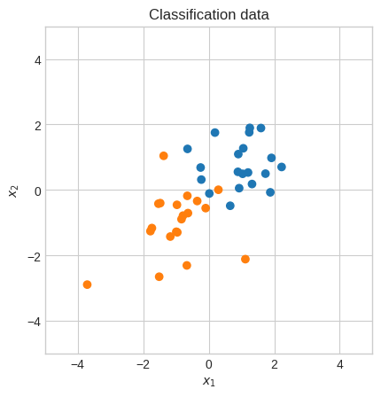
Single-neuron network with sigmoid activation and Log loss function

As before, let the linear model \(Z = wX + b\) and \(Y\) a row vector containing the labels of \(m\) samples.

m = 40
k = 2
neg_centroid = [-1, -1]
pos_centroid = [1, 1]

rng = np.random.default_rng(1)
X = np.r_[
    rng.standard_normal((m // 2, k)) + neg_centroid,
    rng.standard_normal((m // 2, k)) + pos_centroid,
].T
Y = np.array([[0] * (m // 2) + [1] * (m // 2)])

plt.scatter(X[0], X[1], c=np.where(Y.squeeze() == 0, "tab:orange", "tab:blue"))
plt.gca().set_aspect("equal")
plt.xlabel("$x_1$")
plt.ylabel("$x_2$")
plt.xlim(-5, 5)
plt.ylim(-5, 5)
plt.title("Classification data")
plt.show()

This time, though, the predictions \(\hat{Y}\) are the result of passing \(Z\) to a sigmoid function, so that \(\hat{Y} = \sigma(Z)\).

\(\sigma(Z) = \cfrac{1}{1+e^{-Z}}\)

To visualize the sigmoid function let’s add another axis.

neg_scatter = go.Scatter3d(
    z=np.full(int(m / 2), 0),
    x=X[0, : int(m / 2)],
    y=X[1, : int(m / 2)],
    mode="markers",
    marker=dict(color="#ff7f0e", size=5),
    name="negative class",
)
pos_scatter = go.Scatter3d(
    z=np.full(int(m / 2), 1),
    x=X[0, int(m / 2) :],
    y=X[1, int(m / 2) :],
    mode="markers",
    marker=dict(color="#1f77b4", size=5),
    name="positive class",
)

fig = go.Figure([pos_scatter, neg_scatter])
fig.update_layout(
    title="Classification data",
    autosize=False,
    width=600,
    height=600,
    margin=dict(l=10, r=10, b=10, t=30),
    scene=dict(
        xaxis=dict(title="x1", range=[-5, 5]),
        yaxis=dict(title="x2", range=[-5, 5]),
        zaxis_title="y",
        camera_eye=dict(x=0, y=0.3, z=2.5),
        camera_up=dict(x=0, y=np.sin(np.pi), z=0),
    ),
)

Now, let’s plot the predictions of a randomly initialized model.

def sigmoid(x):
    return 1 / (1 + np.exp(-x))


xx1, xx2 = np.meshgrid(np.linspace(-5, 5, 100), np.linspace(-5, 5, 100))
w, b = init_neuron_params(k).values()
random_model_plane = go.Surface(
    z=sigmoid(w[0, 0] * xx1 + w[0, 1] * xx2 + b),
    x=xx1,
    y=xx2,
    colorscale=[[0, "#ff7f0e"], [1, "#1f77b4"]],
    showscale=False,
    opacity=0.5,
    name="init params",
)
fig.add_trace(random_model_plane)
fig.update_layout(
    title="Random model",
)
fig.show()

It turns out that the output of the sigmoid activation is the probability \(p\) of a sample belonging to the positive class, which implies that \((1-p)\) is the probability of a sample belonging to the negative class.

Intuitively, a loss function will be small when \(p_i\) is close to 1.0 and \(y_i = 1\) and when \(p_i\) is close to 0.0 and \(y_i = 0\).

For a single sample this loss function might look like this

\(\ell(w, b, y_i) = -p_i^{y_i}(1-p_i)^{1-y_i}\)

For the whole sample the loss would be

\(\mathcal{L}(w, b, Y) = -\prod \limits_{i=1}^{m} p_i^{y_i}(1-p_i)^{1-y_i}\)

In Univariate optimization (week 1) we’ve seen how it’s easier to calculate the derivative of the logarithm of the PMF of the Binomial Distribution.

We can do the same here to obtain a more manageable loss function.

\(\mathcal{L}(w, b, Y) = -\sum \limits_{i=1}^{m} y_i \ln p_i + (1-y_i) \ln (1-p_i)\)

It turns out it’s standard practice to minimize a function and to average the loss over the sample (to manage the scale of the loss for large datasets), so we’ll use this instead:

\(\mathcal{L}(w, b, Y) = -\cfrac{1}{m} \sum \limits_{i=1}^{m} y_i \ln p_i + (1-y_i) \ln (1-p_i)\)

Finally, let’s substitute back \(\hat{y}_i\) for \(p_i\).

\(\mathcal{L}(w, b, Y) = -\cfrac{1}{m} \sum \limits_{i=1}^{m} y_i \ln \hat{y}_i + (1-y_i) \ln (1-\hat{y}_i)\)

Recall that \(\hat{y}_i = \sigma(z_i)\).

def compute_log_loss(Y, Y_hat):
    m = Y_hat.shape[1]
    loss = (-1 / m) * (
        np.dot(Y, np.log(Y_hat).T) + np.dot((1 - Y), np.log(1 - Y_hat).T)
    )
    return loss.squeeze()


params = init_neuron_params(k)
Y_hat = neuron_output(X, params, sigmoid)
print(f"Log loss of random model: {compute_log_loss(Y, Y_hat):.2f}")

Log loss of random model: 0.50

The partial derivatives of the loss function are

\(\cfrac{\partial \mathcal{L}}{\partial w} = \cfrac{\partial \mathcal{L}}{\partial \hat{Y}}\cfrac{\partial \hat{Y}}{\partial w}\)

\(\cfrac{\partial \mathcal{L}}{\partial b} = \cfrac{\partial \mathcal{L}}{\partial \hat{Y}}\cfrac{\partial \hat{Y}}{\partial b}\)

Because we have an activation function around \(Z\), we have another chain rule to apply.

For the MSE loss, the activation was an identity function so it didn’t pose the same challenge.

\(\cfrac{\partial \mathcal{L}}{\partial w} = \cfrac{\partial \mathcal{L}}{\partial \sigma(Z)}\cfrac{\partial \sigma(Z)}{\partial w} = \cfrac{\partial \mathcal{L}}{\partial \sigma(Z)}\cfrac{\partial \sigma(Z)}{\partial Z}\cfrac{\partial Z}{\partial w}\)

\(\cfrac{\partial \mathcal{L}}{\partial b} = \cfrac{\partial \mathcal{L}}{\partial \sigma(Z)}\cfrac{\partial \sigma(Z)}{\partial b} = \cfrac{\partial \mathcal{L}}{\partial \sigma(Z)}\cfrac{\partial \sigma(Z)}{\partial Z}\cfrac{\partial Z}{\partial b}\)

Let’s calculate \(\cfrac{\partial \mathcal{L}}{\partial \sigma(Z)}\), \(\cfrac{\partial \sigma(Z)}{\partial Z}\), \(\cfrac{\partial Z}{\partial w}\) and \(\cfrac{\partial Z}{\partial b}\)

Calculation of partial derivative of Log loss wrt sigmoid activation

\(\cfrac{\partial \mathcal{L}}{\partial \sigma(Z)} = \cfrac{\partial}{\partial \sigma(Z)} -\cfrac{1}{m} \sum \limits_{i=1}^{m} Y\ln\sigma(Z)+(Y-1)\ln(1-\sigma(Z))\)

\(= -\cfrac{1}{m} \sum \limits_{i=1}^{m} \cfrac{Y}{\sigma(Z)}+\cfrac{Y-1}{1-\sigma(Z)}\)

\(= -\cfrac{1}{m} \sum \limits_{i=1}^{m} \cfrac{Y(1-\sigma(Z)) + (Y-1)\sigma(Z)}{\sigma(Z)(1-\sigma(Z))}\)

\(= -\cfrac{1}{m} \sum \limits_{i=1}^{m} \cfrac{Y -\sigma(Z)}{\sigma(Z)(1-\sigma(Z))}\)

Calculation of the derivative of the sigmoid function

\(\cfrac{\partial \sigma(Z)}{\partial Z} = \cfrac{\partial}{\partial Z} \cfrac{1}{1+e^{-Z}}\)

\(= (1+e^{-Z})^{-1}\)

\(= -(1+e^{-Z})^{-2}(-e^{-Z})\)

\(= (1+e^{-Z})^{-2}e^{-Z}\)

\(= \cfrac{e^{-Z}}{(1+e^{-Z})^2}\)

\(= \cfrac{1 +e^{-Z} - 1}{(1+e^{-Z})^2}\)

\(= \cfrac{1 +e^{-Z}}{(1+e^{-Z})^2}-\cfrac{1}{(1+e^{-Z})^2}\)

\(= \cfrac{1}{1+e^{-Z}}-\cfrac{1}{(1+e^{-Z})^2}\)

Because the factor of \(x-x^2\) is \(x(1-x)\) we can factor it to

\(= \cfrac{1}{1+e^{-Z}}\left(1 - \cfrac{1}{1+e^{-Z}} \right)\)

\(= \sigma(Z)(1 - \sigma(Z))\)

The other two partial derivatives are the same as the MSE loss’.

\(\cfrac{\partial Z}{\partial w} = \cfrac{\partial}{\partial w} wX+b = X\)

\(\cfrac{\partial Z}{\partial b} = \cfrac{\partial}{\partial b} wX+b = 1\)

Let’s put it all together

\(\cfrac{\partial \mathcal{L}}{\partial w} = -\cfrac{1}{m} \sum \limits_{i=1}^{m} \cfrac{Y -\sigma(Z)}{\sigma(Z)(1-\sigma(Z))} \sigma(Z)(1 - \sigma(Z)) X^T = -\cfrac{1}{m} \sum \limits_{i=1}^{m} (Y -\sigma(Z))X^T = -\cfrac{1}{m} \sum \limits_{i=1}^{m} (Y - \hat{Y}) X^T\)

\(\cfrac{\partial \mathcal{L}}{\partial b} = -\cfrac{1}{m} \sum \limits_{i=1}^{m} \cfrac{Y -\sigma(Z)}{\sigma(Z)(1-\sigma(Z))} \sigma(Z)(1 - \sigma(Z)) = -\cfrac{1}{m} \sum \limits_{i=1}^{m} Y - \hat{Y}\)

🔑 The partial derivatives of the Log loss \(\cfrac{\partial \mathcal{L}}{\partial w}\) and \(\cfrac{\partial \mathcal{L}}{\partial b}\) are the same as the MSE loss’.

params = init_neuron_params(k)
Y_hat = neuron_output(X, params, sigmoid)
print(f"Log loss before update: {compute_log_loss(Y, Y_hat):.2f}")
grads = compute_grads(X, Y, Y_hat)
params = update_params(params, grads)
Y_hat = neuron_output(X, params, sigmoid)
print(f"Log loss after update: {compute_log_loss(Y, Y_hat):.2f}")

Log loss before update: 0.53
Log loss after update: 0.51

Let’s find the best parameters using gradient descent.

params = init_neuron_params(k)
Y_hat = neuron_output(X, params, sigmoid)
loss = compute_log_loss(Y, Y_hat)
print(f"Iter 0  - Log loss={loss:.6f}")
for i in range(1, 500 + 1):
    grads = compute_grads(X, Y, Y_hat)
    params = update_params(params, grads)
    Y_hat = neuron_output(X, params, sigmoid)
    loss_new = compute_log_loss(Y, Y_hat)
    if loss - loss_new <= 1e-4:
        print(f"Iter {i} - Log loss={loss:.6f}")
        print("The algorithm has converged")
        break
    loss = loss_new
    if i % 100 == 0:
        print(f"Iter {i} - Log loss={loss:.6f}")

Iter 0  - Log loss=0.582076
Iter 100 - Log loss=0.182397
Iter 200 - Log loss=0.148754
Iter 300 - Log loss=0.134595
Iter 306 - Log loss=0.134088
The algorithm has converged

Let’s visualize the final model.

w, b = params.values()
final_model_plane = go.Surface(
    z=sigmoid(w[0, 0] * xx1 + w[0, 1] * xx2 + b),
    x=xx1,
    y=xx2,
    colorscale=[[0, "#ff7f0e"], [1, "#1f77b4"]],
    showscale=False,
    opacity=0.5,
    name="final params",
)
fig.add_trace(final_model_plane)
fig.data[2].visible = False
fig.update_layout(title="Final model")
fig.show()

Neural network with 1 hidden layer of 3 neurons and sigmoid activations

Motivation

Let’s create non-linear classification data to see the shortcomings of the previous model.

m = 100
k = 2
linspace_out = np.linspace(0, 2 * np.pi, m // 2, endpoint=False)
linspace_in = np.linspace(0, 2 * np.pi, m // 2, endpoint=False)
outer_circ_x = np.cos(linspace_out)
outer_circ_y = np.sin(linspace_out)
inner_circ_x = np.cos(linspace_in) * 0.3
inner_circ_y = np.sin(linspace_in) * 0.3

rng = np.random.default_rng(1)
X = np.vstack(
    [np.append(outer_circ_x, inner_circ_x), np.append(outer_circ_y, inner_circ_y)]
)
X += rng.normal(scale=0.1, size=X.shape)
X = (X - np.mean(X, axis=1, keepdims=True)) / np.std(X, axis=1, keepdims=True)
Y = np.array([[0] * (m // 2) + [1] * (m // 2)])

plt.scatter(X[0], X[1], c=np.where(Y.squeeze() == 0, "tab:orange", "tab:blue"))
plt.gca().set_aspect("equal")
plt.xlabel("$x_1$")
plt.ylabel("$x_2$")
plt.xlim(-3, 3)
plt.ylim(-3, 3)
plt.title("Non-linear classification data")
plt.show()

As before let’s add another axis to visualize the model.

neg_scatter = go.Scatter3d(
    z=np.full(int(m / 2), 0),
    x=X[0, : int(m / 2)],
    y=X[1, : int(m / 2)],
    mode="markers",
    marker=dict(color="#ff7f0e", size=5),
    name="negative class",
)
pos_scatter = go.Scatter3d(
    z=np.full(int(m / 2), 1),
    x=X[0, int(m / 2) :],
    y=X[1, int(m / 2) :],
    mode="markers",
    marker=dict(color="#1f77b4", size=5),
    name="positive class",
)

fig = go.Figure([pos_scatter, neg_scatter])
fig.update_layout(
    title="Non-linear classification data",
    autosize=False,
    width=600,
    height=600,
    margin=dict(l=10, r=10, b=10, t=30),
    scene=dict(
        xaxis=dict(title="x1", range=[-3, 3]),
        yaxis=dict(title="x2", range=[-3, 3]),
        zaxis_title="y",
        aspectmode="cube",
        camera_eye=dict(x=0, y=0, z=2.5),
        camera_up=dict(x=0, y=np.sin(np.pi), z=0),
    ),
)

Let’s train a single-neuron model with sigmoid activation using a Log loss function and plot the respective plane.

params = init_neuron_params(k)
Y_hat = neuron_output(X, params, sigmoid)
loss = compute_log_loss(Y, Y_hat)
print(f"Iter 0  - Log loss={loss:.6f}")
for i in range(1, 500 + 1):
    grads = compute_grads(X, Y, Y_hat)
    params = update_params(params, grads)
    Y_hat = neuron_output(X, params, sigmoid)
    loss_new = compute_log_loss(Y, Y_hat)
    if loss - loss_new <= 1e-4:
        print(f"Iter {i} - Log loss={loss:.6f}")
        print("The algorithm has converged")
        break
    loss = loss_new
    if i % 100 == 0:
        print(f"Iter {i} - Log loss={loss:.6f}")

w, b = params.values()
xx1, xx2 = np.meshgrid(np.linspace(-2, 2, 100), np.linspace(-2, 2, 100))
final_model_plane = go.Surface(
    z=sigmoid(w[0, 0] * xx1 + w[0, 1] * xx2 + b),
    x=xx1,
    y=xx2,
    colorscale=[[0, "#ff7f0e"], [1, "#1f77b4"]],
    showscale=False,
    opacity=0.5,
    name="final params",
)
fig.add_trace(final_model_plane)
fig.update_layout(
    title="Linear model on non-linear data",
)
fig.show()

Iter 0  - Log loss=0.732818
Iter 62 - Log loss=0.695059
The algorithm has converged

Let’s try to improve it by adding more neurons.

Neural network notation

The neural network we will be building is shown below.

A note on the indices of the weights:

For example, \(w_{121}\) (\(w_{\text{AT },\text{FROM },\text{TO}}\)) means “weight AT layer 1, FROM node 2 (previous layer) TO node 1 (current layer)”.

Let \(Z_1\) the \((n, m)\) pre-activation matrix of the first and only hidden layer.

\(Z_1 = \begin{bmatrix} w_{111}x_{11}+w_{121}x_{21}+b_{1}&& w_{111}x_{12}+w_{121}x_{22}+b_{1}&& \cdots&& w_{111}x_{1m}+w_{121}x_{2m}+b_{1}\\ w_{112}x_{11}+w_{122}x_{21}+b_{1}&& w_{112}x_{12}+w_{122}x_{22}+b_{1}&& \cdots&& w_{112}x_{1m}+w_{122}x_{2m}+b_{1}\\ w_{113}x_{11}+w_{123}x_{21}+b_{1}&& w_{113}x_{12}+w_{123}x_{22}+b_{1}&& \cdots&& w_{113}x_{1m}+w_{123}x_{2m}+b_{1} \end{bmatrix}\)

A more compact matrix notation is shown below.

\(Z_1 = \begin{bmatrix} w_{111}&&w_{121}\\ w_{112}&&w_{122}\\ w_{113}&&w_{123}\\ \end{bmatrix} \begin{bmatrix} x_{11}&&x_{12}&&\cdots&&x_{1m}\\ x_{21}&&x_{22}&&\cdots&&x_{2m} \end{bmatrix} + \begin{bmatrix}b_{1}\end{bmatrix}\)

Let \(A_1 = h(Z_1)\) where \(h\) is an activation function (eg linear, sigmoid). For the hidden layers it’s common to use other a ReLU activation function.

Let \(Z_2\) a \((3, m)\) pre-activation matrix of the output layer.

\(Z_2 = \begin{bmatrix}w_{211}&&w_{221}&&w_{231}\end{bmatrix} \begin{bmatrix} a_{111}&&a_{112}&&\dots&&a_{11m}\\ a_{121}&&a_{122}&&\dots&&a_{12m}\\ a_{131}&&a_{132}&&\dots&&a_{13m} \end{bmatrix} + \begin{bmatrix}b_{2}\end{bmatrix}\)

\(\hat{Y} = \sigma(Z_2)\)

Note that we could use \(a_{0km}\) instead of \(x_{km}\) if we want to define a generic \(Z_{LAYER}\) matrix, but it’s better to keep \(x\) and \(a\) distinct although it can help thinking that \(x\) is basically just \(a_0\).

Partial derivatives of a neural network

In our network we need 5 steps to go from the inputs through the hidden layer to the loss function.

For 1 sample (omitting the \(i\) index for conciseness):

1. calculate the linear combinations \(z_{1n}\) for all \(n\) neurons in the first hidden layer.

\(z_{1n} = w_{11n}x_1 + w_{12n}x_2 + b_1\)

2. pass them to the sigmoid activation function

\(a_{1n} = \sigma(z_{1n})\)

3. calculate the linear combination \(z_{21}\) for the final output node

\(z_{21} = w_{211}a_{11} + w_{221}a_{12} + w_{231}a_{13} + b_2\)

4. pass it to the sigmoid activation function

\(\hat{Y} = \sigma(z_{21})\)

5. compute the Log loss

\(\mathcal{L}(w, b, Y) = -y \ln \hat{y} + (1-y) \ln (1-\hat{y})\)

It turns out that to work out the chain rule of the partial derivative of the loss wrt to a parameter of an input node we just need to chain the partial derivatives of these 5 functions.

For example, let’s workout the chain rule for \(\cfrac{\partial \mathcal{L}}{\partial w_{111}}\)

Moving backwards, the first derivative we encounter is at 5. \(\cfrac{\partial \mathcal{L}}{\partial \hat{Y}}\), then at 4. \(\cfrac{\partial \hat{Y}}{\partial z_{21}}\), then at 3. \(\cfrac{\partial z_{21}}{\partial a_{11}}\), then at 2. \(\cfrac{\partial a_{11}}{\partial z_{11}}\) and finally at 1. \(\cfrac{\partial z_{11}}{\partial w_{111}}\)

\(\cfrac{\partial \mathcal{L}}{\partial w_{111}} = \cfrac{\partial \mathcal{L}}{\partial \hat{Y}} \cfrac{\partial \hat{Y}}{\partial z_{21}} \cfrac{\partial z_{21}}{\partial a_{11}} \cfrac{\partial a_{11}}{\partial z_{11}} \cfrac{\partial z_{11}}{\partial w_{111}}\)

From Calculation of partial derivative of Log loss wrt sigmoid activation we know

\(\cfrac{\partial \mathcal{L}}{\partial \hat{Y}} = -\cfrac{Y - \hat{Y}}{\hat{Y}(1-\hat{Y})}\)

From Calculation of the derivative of the sigmoid function we know

\(\cfrac{\partial \hat{Y}}{\partial z_{21}} = \hat{Y}(1-\hat{Y})\)

And we know that these two simplify to

\(\cfrac{\partial \mathcal{L}}{\partial \hat{Y}}\cfrac{\partial \hat{Y}}{\partial z_{21}} = - (Y - \hat{Y})\)

Similarly to \(\cfrac{\partial \hat{Y}}{\partial z_{21}}\) (partial derivative of the sigmoid function in the output node wrt its argument) we obtain \(\cfrac{\partial a_{11}}{\partial z_{11}}\) (partial derivative of the sigmoid function in the first node of the hidden layer wrt its argument)

\(\cfrac{\partial a_{11}}{\partial z_{11}} = a_{11}(1-a_{11})\)

Then the others are very easy to calculate.

\(\cfrac{\partial z_{21}}{\partial a_{11}} = \cfrac{\partial}{\partial a_{11}} w_{211}a_{11} + w_{221}a_{12} + w_{231}a_{13} + b_2 = w_{211}\)

\(\cfrac{\partial z_{11}}{\partial w_{111}} = \cfrac{\partial}{\partial w_{111}} w_{111}x_1 + w_{121}x_2 + b_1 = x_1\)

Let’s put it all together.

\(\cfrac{\partial \mathcal{L}}{\partial w_{111}} = - (Y - \hat{Y})w_{211}a_{11}(1-a_{11})x_1\)

The partial derivative of the loss wrt of the weights in the hidden layer are the same as when we had a single-neuron neural network.

As an example, let’s calculate \(\cfrac{\partial \mathcal{L}}{\partial w_{231}}\).

\(\cfrac{\partial \mathcal{L}}{\partial w_{231}} = \cfrac{\partial \mathcal{L}}{\partial \hat{Y}} \cfrac{\partial \hat{Y}}{\partial z_{21}} \cfrac{\partial z_{21}}{\partial w_{231}}\)

The only one we need to calculate is

\(\cfrac{\partial z_{21}}{\partial w_{231}} = \cfrac{\partial}{\partial w_{231}}w_{211}a_{11} + w_{221}a_{12} + w_{231}a_{13} + b_2 = a_{13}\)

Let’s put it all together.

\(\cfrac{\partial \mathcal{L}}{\partial w_{231}} = - (Y - \hat{Y})a_{13}\)

Forward and backward propagation

It turns out there is an algorithm to efficiently train a neural network.

🔑 Forward propagation refers to the calculation and storage of output layers for backward propagation

🔑 Backward propagation (aka backprop) refers to the calculation of partial derivatives for each layer where hidden layers both output the partial derivative of the loss wrt to the parameters used in the layer but also the partial derivative of the loss wrt the output of the previous layer

Forward propagation doesn’t need a lot of explanation. A key aspect, though, is the storage of the outputs.

Backward propagation is also quite intuitive at the very high level as that’s sort of how, for example, we naturally approached the chain rule of \(\cfrac{\partial \mathcal{L}}{\partial w_{111}}\).

Recall we moved backwards starting from the partial derivative of the loss wrt to \(\hat{Y}\) and we ended up with

\(\cfrac{\partial \mathcal{L}}{\partial w_{111}} = \cfrac{\partial \mathcal{L}}{\partial \hat{Y}} \cfrac{\partial \hat{Y}}{\partial z_{21}} \cfrac{\partial z_{21}}{\partial a_{11}} \cfrac{\partial a_{11}}{\partial z_{11}} \cfrac{\partial z_{11}}{\partial w_{111}}\)

The forward and backward propagation algorithm is shown below.

Note how the partial derivative of the loss wrt the parameters is built progressively and carried over from one layer to the next (or previous depends on how you look at it).

The gray bit of the chain rule is what’s been carried over and the black bit is what’s been appended at each step.

Also note how the process “drops” the partial derivative of the loss wrt the parameters for the final layer as it goes, while it keeps building the partial derivative for the parameters used in the first layer.

That’s the main idea behind its efficiency.

The backward propagation for a network like the one we will be building will look like this.

Step 1

Inputs: \(Y\), \(\hat{Y}\)

compute \(\cfrac{\partial \mathcal{L}}{\partial \hat{Y}} = -\cfrac{Y - \hat{Y}}{\hat{Y}(1-\hat{Y})}\)

Outputs: \(\cfrac{\partial \mathcal{L}}{\partial \hat{Y}}\) (carry over to the next step)

Step 2

Inputs: \(\cfrac{\partial \mathcal{L}}{\partial \hat{Y}}\) (from previous step), \(A_1\), \(W_2\), \(Z_2\) (from the layer’s cache)

compute \(\cfrac{\partial \hat{Y}}{\partial Z_{2}} = \cfrac{\partial}{\partial Z_{2}}\sigma(Z_2)\)

compute \(\cfrac{\partial \mathcal{L}}{\partial Z_{2}} = \cfrac{\partial \mathcal{L}}{\partial \hat{Y}}\cfrac{\partial \hat{Y}}{\partial Z_{2}}\)

compute \(\cfrac{\partial \mathcal{L}}{\partial A_{1}} = W_2^T \cdot \cfrac{\partial \mathcal{L}}{\partial Z_{2}}\)

compute \(\cfrac{\partial \mathcal{L}}{\partial W_{2}} = \cfrac{1}{m} \sum \limits_{i=1}^{m} \cfrac{\partial \mathcal{L}}{\partial Z_{2}} \cdot A_1^T\)

compute \(\cfrac{\partial \mathcal{L}}{\partial b_{2}} = \cfrac{1}{m} \sum \limits_{i=1}^{m} \cfrac{\partial \mathcal{L}}{\partial Z_{2}}\)

Outputs: \(\cfrac{\partial \mathcal{L}}{\partial A_{1}}\) (carry over to the next step), \(\cfrac{\partial \mathcal{L}}{\partial W_{2}}\), \(\cfrac{\partial \mathcal{L}}{\partial b_{2}}\) (send to update params process)

Step 3

Inputs: \(\cfrac{\partial \mathcal{L}}{\partial A_{1}}\) (from the previous step), \(X\), \(W_1\), \(Z_1\) (from the layer’s cache)

compute \(\cfrac{\partial A_{1}}{\partial Z_{1}} = \cfrac{\partial}{\partial Z_{1}}\text{ReLU}(Z_1)\)

compute \(\cfrac{\partial \mathcal{L}}{\partial Z_{1}} = \cfrac{\partial \mathcal{L}}{\partial \hat{Y}}\cfrac{\partial A_{1}}{\partial Z_{1}}\)

compute \(\cfrac{\partial \mathcal{L}}{\partial X} = W_1^T \cdot \cfrac{\partial \mathcal{L}}{\partial Z_{1}}\)

compute \(\cfrac{\partial \mathcal{L}}{\partial W_{1}} = \cfrac{1}{m} \sum \limits_{i=1}^{m} \cfrac{\partial \mathcal{L}}{\partial Z_{1}} \cdot X^T\)

compute \(\cfrac{\partial \mathcal{L}}{\partial b_{1}} = \cfrac{1}{m} \sum \limits_{i=1}^{m} \cfrac{\partial \mathcal{L}}{\partial Z_{1}}\)

Outputs: \(\cfrac{\partial \mathcal{L}}{\partial A_{0}}\) (do not use further), \(\cfrac{\partial \mathcal{L}}{\partial W_{1}}\), \(\cfrac{\partial \mathcal{L}}{\partial b_{1}}\) (send to update params process)

More generally, the pseudo-code might be something along these lines.

\(\begin{array}{l} \textbf{Algorithm: } \text{Forward and Backward Propagation} \\ \textbf{Input: } X, Y, \text{initial parameter} [W_1, b_1, \dots, W_L, b_L] \\ \textbf{Output: } \text{gradients} [\nabla W_1, \nabla b_1, \dots, \nabla W_L, \nabla b_L] \\ \phantom{0}1 : L \gets \text{len}([W_1, b_1, \dots, W_L, b_L]) / 2 \\ \phantom{0}2 : A_{i-1} \gets X \\ \phantom{0}3 : \text{Forward propagation:} \\ \phantom{0}4 : \text{for i = 1 to L do} \\ \phantom{0}5 : \quad \text{if } i < L \text{ then} \\ \phantom{0}6 : \quad \quad \mathcal{f}_i \gets ReLU \\ \phantom{0}7 : \quad \text{else } \\ \phantom{0}8 : \quad \quad \mathcal{f}_i \gets \sigma \\ \phantom{0}9 : \quad \text {end if} \\ 10 : \quad Z_i \gets W_iA_{i-1} + b_i \\ 11 : \quad A_i \gets \mathcal{f}_i(Z_i) \\ 12 : \quad \text{cache}_i \gets [A_{i-1}, \mathcal{f}_i, W_i, Z_i] \\ 13 : \quad \text{if } i = L \text{ then} \\ 14 : \quad \quad \hat{Y} \gets A_L \\ 15 : \quad \text {end if} \\ 16 : \text{end for} \\ 17 : \text{Backward propagation:} \\ 18 : dA_L \gets -(Y - \hat{Y}) / \hat{Y}(1-\hat{Y}) \\ 19 : \text{for i = L down to 1 do} \\ 20 : \quad [A_{i-1}, \mathcal{f}_i, W_i, Z_i] \gets \text{unpack } \text{cache}_i \\ 21 : \quad dZ_i = dA_i \mathcal{f'}_i(Z_i) \\ 22 : \quad \nabla W_i = (1/m) \sum_{i=1}^{m} dZ_i A_{i-1}^T \\ 23 : \quad \nabla b_i = (1/m) \sum_{i=1}^{m} dZ_i \\ 24 : \quad dA_{i-1} = W_i^T dZ_i \\ 25 : \text{end for} \\ 26 : \text{return } [\nabla W_1, \nabla b_1, \dots, \nabla W_L, \nabla b_L] \\ \end{array}\)

Building a neural network

The first step is to randomly initialize all the parameters.

A common initialization of weights in neural networks is the Glorot Uniform, which takes into account the size of the previous layer and the size of the current layer.

\(W_{i} \sim U\left(-\cfrac{\sqrt{6}}{\sqrt{fan_{i-1} + fan_{i}}}, \cfrac{\sqrt{6}}{\sqrt{fan_{i-1} + fan_{i}}}\right)\), where \(U(a, b)\) is the Uniform distribution and \(fan_{i-1}\) is the size of the previous layer and \(fan_i\) is the size of the current layer.

def init_nn_params(n):
    params = {}
    for i in range(len(n) - 1):
        fan_in, fan_out = n[i : i + 2]
        limit = np.sqrt(6 / (fan_in + fan_out))
        params["W" + str(i + 1)] = rng.uniform(-limit, limit, size=(fan_out, fan_in))
        params["b" + str(i + 1)] = np.zeros((n[i + 1], 1))
    return params


params = init_nn_params([X.shape[0], 3, Y.shape[0]])
params

{'W1': array([[ 0.223084  , -0.4653109 ],
        [ 0.61949715, -0.54494543],
        [-0.93066582,  1.01408548]]),
 'b1': array([[0.],
        [0.],
        [0.]]),
 'W2': array([[0.09800704, 0.67090127, 0.07158097]]),
 'b2': array([[0.]])}

Then, we do forward propagation and compute the loss.

def relu(x):
    # np.maximum: element-wise max, not np.max along axis
    return np.maximum(0, x)


def step_forward_prop(A_prev, layer, params, activation):
    W = params["W" + str(layer)]
    b = params["b" + str(layer)]
    Z = W @ A_prev + b
    A = activation(Z)
    cache = A_prev, W, Z, activation.__name__
    return A, cache


def forward_prop(X, params, hidden_activation=relu, ouput_activation=sigmoid):
    A_prev = X
    caches = []
    n_layers = len(params) // 2
    for layer in range(1, n_layers + 1):
        if layer <= n_layers - 1:
            activation = hidden_activation
        else:
            activation = ouput_activation
        A, cache = step_forward_prop(A_prev, layer, params, activation)
        A_prev = A
        caches.append(cache)
    return A, caches


Y_hat, caches = forward_prop(X, params)
print(f"Output layer is {caches[-1][2].shape} with {caches[-1][3]} activation")
for layer in range(len(caches) - 2, -1, -1):
    print(
        f"Hidden layer {layer + 1} is {caches[layer][2].shape} with {caches[layer][3]} activation"
    )
print(f"\nLog loss of random model: {compute_log_loss(Y, Y_hat):.2f}")

Output layer is (1, 100) with sigmoid activation
Hidden layer 1 is (3, 100) with relu activation

Log loss of random model: 0.79

Then, we do backward propagation.

In Proof that ReLU is not differentiable at 0 we said that the convention in machine learning is to consider its derivative at 0, well, 0.

Let’s see how just one undetermined derivative can wreak havoc on the parameters gradients during backward propagation.

def d_sigmoid(x):
    return sigmoid(x) * (1 - sigmoid(x))


def d_relu(x):
    if isinstance(x, np.ndarray):
        x = x.copy()
        x[x == 0] = np.nan
    elif x == 0:
        x = np.nan
    return np.sign(relu(x))


dA2 = -(Y - Y_hat) / np.multiply(Y_hat, (1 - Y_hat))
A1, W2, Z2, _ = caches[1]
dZ2 = dA2 * d_sigmoid(Z2)
dA1 = np.dot(W2.T, dZ2)
X, W1, Z1, _ = caches[0]
# let's introduce one NaN in Z1
Z1[0, 0] = np.nan
dZ1 = dA1 * d_relu(Z1)
dW1 = (1 / dZ1.shape[1]) * np.dot(dZ1, X.T)
dW1 = dW1.round(2)

display(
    Math(
        "\\langle \\nabla W_{111}, \\nabla W_{121} \\rangle="
        + sp.latex(sp.Matrix(dW1[0]))
    ),
    Math(
        "\\langle \\nabla W_{112}, \\nabla W_{122} \\rangle="
        + sp.latex(sp.Matrix(dW1[1]))
    ),
    Math(
        "\\langle \\nabla W_{113}, \\nabla W_{123} \\rangle="
        + sp.latex(sp.Matrix(dW1[2]))
    ),
)

$\displaystyle \langle \nabla W_{111}, \nabla W_{121} \rangle=\left[\begin{matrix}\text{NaN}\\\text{NaN}\end{matrix}\right]$

$\displaystyle \langle \nabla W_{112}, \nabla W_{122} \rangle=\left[\begin{matrix}0.09\\-0.07\end{matrix}\right]$

$\displaystyle \langle \nabla W_{113}, \nabla W_{123} \rangle=\left[\begin{matrix}-0.01\\0.01\end{matrix}\right]$

So we can’t simply do this.

\(\cfrac{\partial A_{1}}{\partial Z_{1}} = \cfrac{\partial}{\partial Z_{1}}\text{ReLU}(Z_1) = \begin{cases}1 \text{ if } x > 0\\0 \text{ if } x < 0\\\text{undefined if } x = 0\end{cases}\)

As per the convention, we’ll do this instead.

\(\cfrac{\partial A_{1}}{\partial Z_{1}} = \begin{cases}1 \text{ if } x > 0\\0 \text{ if } x \le 0\end{cases}\)

def init_backward_prop(Y_hat):
    dAL = -(Y - Y_hat) / np.multiply(Y_hat, (1 - Y_hat))
    return dAL


def step_backward_prop(dA_prev, cache):
    # extract elements from cache
    A_prev, W, Z, activation = cache
    # propagate dA gradient through activation function
    # d_relu is nan when x is 0
    # instead of propagating nan's we make them 0
    func = {"sigmoid": d_sigmoid, "relu": lambda x: np.nan_to_num(d_relu(x))}
    dZ = dA_prev * func[activation](Z)
    # compute dW, db, dA_prev
    # dZ2 is (1, m) and A1 is (3, m), so dW1 is (1, 3)
    # dZ1 is (3, m) and X is (2, m), so dW0 is (3, 2)
    dW = (1 / dZ.shape[1]) * np.dot(dZ, A_prev.T)
    # dZ2 is (1, m) so db2 is (1, 1)
    # dZ1 is (3, m) so db0 is (1, 3)
    db = (1 / dZ.shape[1]) * np.sum(dZ, axis=1, keepdims=True)
    # W1 is (1, 3) and dZ2 is (1, m), so dA1 is (1, m)
    # W0 is (3, 2) and dZ1 is (3, m), so dX is (3, m) (not used though)
    dA_next = np.dot(W.T, dZ)
    return dA_next, dW, db


def backward_prop(Y_hat, caches):
    dA_prev = init_backward_prop(Y_hat)
    grads = params.copy()
    for layer in range(len(caches), 0, -1):
        dA, dW, db = step_backward_prop(dA_prev, caches[layer - 1])
        grads["W" + str(layer)] = dW
        grads["b" + str(layer)] = db
        dA_prev = dA
    return grads


grads = backward_prop(Y_hat, caches)
grads

{'W1': array([[ 0.00495321, -0.01516951],
        [ 0.08724881, -0.07424792],
        [-0.00585036,  0.00528136]]),
 'b1': array([[ 0.00469289],
        [ 0.04855939],
        [-0.00072097]]),
 'W2': array([[0.0867413 , 0.14087237, 0.15088486]]),
 'b2': array([[0.06738911]])}

At this point it’s the usual gradient descent algorithm.

Let’s run it 5 times (each with up to 500 iterations of gradient descent) and pick the run with the lowest training loss.

runs = []
for _ in range(5):
    history = ""
    params = init_nn_params([X.shape[0], 3, Y.shape[0]])
    Y_hat, caches = forward_prop(X, params)
    loss = compute_log_loss(Y, Y_hat)
    history += f"Iter 0   - Log loss={loss:.6f}\n"
    for i in range(1, 500 + 1):
        grads = backward_prop(Y_hat, caches)
        params = update_params(params, grads, learning_rate=0.5)
        Y_hat, caches = forward_prop(X, params)
        loss_new = compute_log_loss(Y, Y_hat)
        if loss - loss_new <= 1e-4:
            history += f"Iter {i} - Log loss={loss:.6f}\n"
            history += f"The algorithm has converged\n"
            break
        loss = loss_new
        if i % 100 == 0:
            history += f"Iter {i} - Log loss={loss:.6f}\n"
    runs.append((loss, params, history))

runs.sort(key=lambda x: x[0])
params = runs[0][1]
print(runs[0][2])

Iter 0   - Log loss=0.618392
Iter 100 - Log loss=0.137058
Iter 200 - Log loss=0.054018
Iter 300 - Log loss=0.033291
Iter 334 - Log loss=0.029567
The algorithm has converged

Let’s visualize the model.

XX = np.c_[xx1.flatten(), xx2.flatten()].T
Y_hat, _ = forward_prop(XX, params)

final_model_plane = go.Surface(
    z=Y_hat.reshape(xx1.shape),
    x=xx1,
    y=xx2,
    colorscale=[[0, "#ff7f0e"], [1, "#1f77b4"]],
    showscale=False,
    opacity=0.5,
    name="final params",
)
fig.data[2].visible = False
fig.add_trace(final_model_plane)
fig.update_layout(
    title="Neural Network model",
)
fig.show()

Newton-Raphson method

Newton-Raphson method with one variable

🔑 Newton-Raphson method is an algorithm to find the zero of a function

It can be used to optimize a function \(f(x)\) by finding the zero of \(f'(x)\).

The method works by starting from a random point \(x_0\) on \(f'(x)\), finding the tangent at \(f'(x_0)\) and finding where the tangent crosses the x-axis.

The idea is that this new point is closer than \(x_0\) to a minimum or maximum.

def fixup_animation_js(html_animation):
    html_animation = html_animation.replace(
        '<div class="anim-controls">',
        '<div class="anim-controls" style="display:none">',
    )
    animation_id = re.findall(r"onclick=\"(.*)\.", html_animation)[0]
    img_id = re.findall(r"<img id=\"(.*)\"", html_animation)[0]
    html_animation += f"""
<script language="javascript">
setupAnimationIntersectionObserver('{animation_id}', '{img_id}');
</script>
"""
    return html_animation


def _update(frame):
    global fscat, dscat, dtang
    fscat.remove()
    dscat.remove()
    dtang.remove()
    fscat = ax.scatter(xs[frame], f(xs[frame]), color="tab:blue")
    dscat = ax.scatter(xs[frame], df(xs[frame]), color="tab:orange")
    (dtang,) = ax.plot(
        xx,
        ddf(xs[frame]) * (xx - xs[frame]) + df(xs[frame]),
        "--",
        color="tab:orange",
        alpha=0.5,
    )


x = sp.symbols("x")
f = sp.exp(x) - sp.log(x)
df = sp.lambdify(x, sp.diff(f, x, 1))
ddf = sp.lambdify(x, sp.diff(f, x, 2))
f = sp.lambdify(x, f)

xs = [1.75]
for _ in range(4):
    xs.append(xs[-1] - df(xs[-1]) / ddf(xs[-1]))

fig, ax = plt.subplots()
xx = np.linspace(1e-3, 2)
ax.plot(xx, f(xx), color="tab:blue", label="$f(x)$")
ax.plot(xx, df(xx), color="tab:orange", label="$f'(x)$")
fscat = ax.scatter([], [])
dscat = ax.scatter([], [])
(dtang,) = ax.plot([], [])
ax.set_ylim(-2, 11)
ax.set_xlim(0, 2)
ax.spines[["left", "bottom"]].set_position(("data", 0))
ax.text(1, 0, "$x$", transform=ax.get_yaxis_transform())
ax.text(0, 1.02, "$f(x)$", transform=ax.get_xaxis_transform())
plt.legend(loc="upper right")
plt.title("Minimazation of $f(x)$ using Newton's method")

ani = FuncAnimation(fig=fig, func=_update, frames=4, interval=1000)
html_animation = ani.to_jshtml(default_mode="loop")
if "runtime" not in get_ipython().config.IPKernelApp.connection_file:
    html_animation = fixup_animation_js(html_animation)
display(HTML(html_animation))
plt.close()

Once Loop Reflect

The equation of a line that passes for \(\left(x_0, f(x_0)\right)\) is the point-slope form

\(f(x) - f(x_0) = m(x-x_0)\)

\(f(x) = m(x - x_0) + f(x_0)\)

We substitute \(f'(x)\) for \(f(x)\), \(f'(x_0)\) for \(f(x_0)\), and the derivative of \(f'(x)\) at \(x_0\) (ie the second derivative \(f''(x_0)\)) for \(m\) and we obtain

\(f'(x) = f''(x_0)(x - x_0) + f'(x_0)\)

Now we want to find the \(x\) such that \(f'(x) = 0\), that is the point where the tangent crosses the x-axis.

\(0 = f''(x_0)(x - x_0) + f'(x_0)\)

\(-f''(x_0)(x - x_0) = f'(x_0)\)

\(-(x - x_0) = \cfrac{f'(x_0)}{f''(x_0)}\)

\(-x + x_0 = \cfrac{f'(x_0)}{f''(x_0)}\)

\(-x = - x_0 + \cfrac{f'(x_0)}{f''(x_0)}\)

\(x = x_0 - \cfrac{f'(x_0)}{f''(x_0)}\)

The pseudo-code might be looking something along these lines

\(\begin{array}{l} \textbf{Algorithm: } \text{Newton's Method for Univariate Optimization} \\ \textbf{Input: } \text{function to minimize } \mathcal{f}, \text{initial guess } x_0, \text{number of iterations } K, \text{convergence } \epsilon \\ \textbf{Output: } x \\ 1 : x \gets x_0 \\ 2 : \text{for k = 1 to K do} \\ 3 : \quad x_{new} = x - f'(x) / f''(x) \\ 4 : \quad \text{if } \|f'(x_{new}) / f''(x_{new})\| < \epsilon \text{ then} \\ 5 : \quad \quad \text{return } x \\ 6 : \quad \text {end if} \\ 7 : \quad x \gets x_{new} \\ 8 : \text{return } x \\ \end{array}\)

Another way to find \(x\) such that \(f'(x) = 0\) is through the rise over run equation.

\(f''(x_0) = \cfrac{f'(x_0)}{x_0 - x}\)

\(\cfrac{1}{f''(x_0)} = \cfrac{x_0 - x}{f'(x_0)}\)

\(\cfrac{f'(x_0)}{f''(x_0)} = x_0 - x\)

\(\cfrac{f'(x_0)}{f''(x_0)} - x_0 = - x\)

\(x_0 - \cfrac{f'(x_0)}{f''(x_0)} = x\)

A third way to find \(x\) such that \(f'(x) = 0\) is through expressing \(f(x)\) as a quadratic approximation (Taylor series truncated at the second order).

A Taylor series of \(f(x)\) that is differentiable at \(x_0\) is

\(f(x)=\sum_{n=0}^\infty\cfrac{f^{(n)}(x_0)(x-x_0)^n}{n!}\)

Before proceeding let’s take a look at what a Taylor series is.

def _update(order):
    global taylor
    taylor.remove()
    series = np.zeros((order, 50))
    for n in range(1, order + 1):
        series[n - 1] = (
            (1 / math.factorial(n))
            * sp.diff(expr, x, n).evalf(subs={x: 0})
            * (xx**n)
        )
    (taylor,) = ax.plot(xx, np.sum(series, axis=0), color="tab:orange")


x = sp.symbols("x")
expr = sp.sin(x)
sin = sp.lambdify(x, expr, "numpy")
xx = np.linspace(-10, 10)
fig, ax = plt.subplots()
ax.plot(xx, sin(xx), color="tab:blue", label="$\sin(x)$")
(taylor,) = ax.plot([], [], color="tab:orange", label="Taylor series")
ax.set_aspect("equal")
ax.set_ylim(-10, 10)
ax.set_xlim(-10, 10)
plt.legend(loc="upper right")
plt.title("Taylor series of order 1, 3, ..., 25 of sine function")


ani = FuncAnimation(fig=fig, func=_update, frames=range(1, 27, 2))
html_animation = ani.to_jshtml(default_mode="loop")
if "runtime" not in get_ipython().config.IPKernelApp.connection_file:
    html_animation = fixup_animation_js(html_animation)
display(HTML(html_animation))
plt.close()

Once Loop Reflect

🔑 The Taylor series of a function is an infinite sum of terms (polynomials) that are expressed in terms of the function derivatives at a point.

The quadratic approximation of \(f(x)\) (Taylor series truncated at the second degree polynomial) is

\(f(x) \approx f(x_0) + f'(x_0)(x-x_0) + \cfrac{1}{2}f''(x_0)(x-x_0)^2\)

To find \(x\) such that \(f'(x) = 0\), we set the derivative of the quadratic approximation to zero.

\(\cfrac{d}{dx}f(x_0) + f'(x_0)(x-x_0) + \cfrac{1}{2}f''(x_0)(x-x_0)^2 = 0\)

\(f'(x_0) + f''(x_0)(x-x_0) = 0\)

\(f''(x_0)(x-x_0) = -f'(x_0)\)

\(x-x_0 = -\cfrac{f'(x_0)}{f''(x_0)}\)

\(x = x_0 -\cfrac{f'(x_0)}{f''(x_0)}\)

This derivation of the Newton’s method update formula from the quadratic approximation of a function has a few important implications:

• At each step, Newton’s method finds the minimum of the quadratic approximation of \(f(x)\)

• When \(f(x)\) is indeed quadratic, Newton’s method will find the minimum or maximum in one single step

• When \(f(x)\) is not quadratic, Newton’s method will exhibit quadratic convergence near the minimum or maximum. Quadratic convergence refers to the rate at which the sequence \({x_k}\) approaches the minimum or maximum. The “error” will decrease quadratically at each step.

def _update(frame):
    global fscat, taylor, taylor_min
    fscat.remove()
    taylor.remove()
    taylor_min.remove()
    fscat = ax.scatter(xs[frame], f(xs[frame]), color="tab:blue")
    (taylor,) = ax.plot(
        xx,
        f(xs[frame])
        + df(xs[frame]) * (xx - xs[frame])
        + (1 / 2) * ddf(xs[frame]) * (xx - xs[frame]) ** 2,
        "--",
        color="tab:orange",
        alpha=0.5,
        label=r"$f(x_0) + f'(x_0)(x-x_0) + \dfrac{1}{2}f''(x_0)(x-x_0)^2$",
    )
    taylor_min = ax.scatter(
        xs[frame + 1],
        f(xs[frame])
        + df(xs[frame]) * (xs[frame + 1] - xs[frame])
        + (1 / 2) * ddf(xs[frame]) * (xs[frame + 1] - xs[frame]) ** 2,
        color="tab:orange",
    )


x = sp.symbols("x")
f = sp.exp(x) - sp.log(x)
df = sp.lambdify(x, sp.diff(f, x, 1))
ddf = sp.lambdify(x, sp.diff(f, x, 2))
f = sp.lambdify(x, f)

xs = [1.75]
for _ in range(4):
    xs.append(xs[-1] - df(xs[-1]) / ddf(xs[-1]))

fig, ax = plt.subplots()
xx = np.linspace(1e-3, 2)
ax.plot(xx, f(xx), color="tab:blue", label="$f(x)$")
fscat = ax.scatter([], [])
(taylor,) = ax.plot(
    [],
    [],
    color="tab:orange",
    alpha=0.5,
    label=r"$f(x_0) + f'(x_0)(x-x_0) + \dfrac{1}{2}f''(x_0)(x-x_0)^2$",
)
taylor_min = ax.scatter([], [])
ax.set_ylim(-2, 11)
ax.set_xlim(0, 2)
ax.spines[["left", "bottom"]].set_position(("data", 0))
ax.text(1, 0, "$x$", transform=ax.get_yaxis_transform())
ax.text(0, 1.02, "$f(x)$", transform=ax.get_xaxis_transform())
plt.legend(loc="upper right")
plt.title(
    "At each step, Newton's method finds\nthe minimum of the quadratic approximation of $f(x)$"
)

ani = FuncAnimation(fig=fig, func=_update, frames=4, interval=1000)
html_animation = ani.to_jshtml(default_mode="loop")
if "runtime" not in get_ipython().config.IPKernelApp.connection_file:
    html_animation = fixup_animation_js(html_animation)
display(HTML(html_animation))
plt.close()

Once Loop Reflect

Finally, let’s inspect the algorithm.

def univariate_newtons_method(f, symbols, initial, steps):
    x = symbols
    df = sp.lambdify(x, sp.diff(f, x, 1))
    ddf = sp.lambdify(x, sp.diff(f, x, 2))
    p = np.zeros((steps, 1))
    g = np.zeros((steps, 1))
    h = np.zeros((steps, 1))
    step_vector = np.zeros((steps, 1))
    p[0] = initial
    g[0] = df(p[0])
    h[0] = ddf(p[0])
    step_vector[0] = df(p[0]) / ddf(p[0])
    for i in range(1, steps):
        p[i] = p[i - 1] - step_vector[i - 1]
        g[i] = df(p[i])
        h[i] = ddf(p[i])
        step_vector[i] = df(p[i]) / ddf(p[i])
        if np.linalg.norm(step_vector[i]) < 1e-4:
            break
    return p[: i + 1], g[: i + 1], h[: i + 1], step_vector[: i + 1]


x = sp.symbols("x")
f = sp.exp(x) - sp.log(x)
p, _, _, _ = univariate_newtons_method(f, symbols=x, initial=1.75, steps=10)
display(
    Math(
        "\\arg \\min \\limits_{x}" + sp.latex(f) + f"={p[-1].squeeze():.4f}"
    )
)
print(f"Newton's method converged after {len(p)-1} steps")

$\displaystyle \arg \min \limits_{x}e^{x} - \log{\left(x \right)}=0.5671$

Newton's method converged after 4 steps

Let’s consider the quadratic function \(f(x) = x^2\) which has a minimum at 0.

Based on what we said above we expect Newton’s method to find this minimum in one step.

x = sp.symbols("x")
f = x**2
p, _, _, _ = univariate_newtons_method(f, symbols=x, initial=1.75, steps=10)
display(
    Math(
        "\\arg \\min \\limits_{x}" + sp.latex(f) + f"={p[-1].squeeze():.4f}"
    )
)
print(f"Newton's method converged after {len(p)-1} steps")

$\displaystyle \arg \min \limits_{x}x^{2}=0.0000$

Newton's method converged after 1 steps

Let’s consider the quadratic function \(f(x) = -x^2\) which has a maximum at 0.

Based on what we said above we expect Newton’s method to find this maximum in one step.

x = sp.symbols("x")
f = -(x**2)
p, _, _, _ = univariate_newtons_method(f, symbols=x, initial=1.75, steps=10)
display(
    Math(
        "\\arg \\min \\limits_{x}"
        + sp.latex(f)
        + f"={p[-1].squeeze():.4f}"
    )
)
print(f"Newton's method converged after {len(p)-1} steps")

$\displaystyle \arg \min \limits_{x}- x^{2}=0.0000$

Newton's method converged after 1 steps

Second derivatives

In the previous section we introduced second derivatives without too much explanation of what they are.

After all, analytically, it’s just the derivative of a derivative.

But what do they represent and what they’re used for?

Consider this analogy.

🔑 Let \(f(t)\) be the distance, then the first derivative is velocity (instantaneous rate of change of distance wrt time), then the second derivative is acceleration (instantaneous rate of change of velocity wrt time).

def _update(raw_frame):
    global distance_point, velocity_point, acceleration_point
    distance_point.remove()
    velocity_point.remove()
    acceleration_point.remove()
    frame = int(frame_func(raw_frame))
    xxf = xx[: frame + 1]
    distance_line = ax.plot(
        xxf, sp.lambdify(x, norm_pdf, "numpy")(xxf), c="tab:blue"
    )
    velocity_line = ax.plot(
        xxf,
        sp.lambdify(x, sp.diff(norm_pdf, x, 1), "numpy")(xxf),
        c="tab:orange",
    )
    acceleration_line = ax.plot(
        xxf,
        sp.lambdify(x, sp.diff(norm_pdf, x, 2), "numpy")(xxf),
        c="tab:green",
    )
    distance_point = ax.scatter(
        xx[frame], sp.lambdify(x, norm_pdf, "numpy")(xx[frame]), color="tab:blue"
    )
    velocity_point = ax.scatter(
        xx[frame],
        sp.lambdify(x, sp.diff(norm_pdf, x, 1), "numpy")(xx[frame]),
        color="tab:orange",
    )
    acceleration_point = ax.scatter(
        xx[frame],
        sp.lambdify(x, sp.diff(norm_pdf, x, 2), "numpy")(xx[frame]),
        color="tab:green",
    )


x = sp.symbols("x")
norm_pdf = (1 / sp.sqrt(2 * np.pi)) * sp.exp(-(x**2) / 2)
xx = np.linspace(-3, 3, 100)
fig, ax = plt.subplots()
distance_line = ax.plot([], [], c="tab:blue", label="distance")
velocity_line = ax.plot([], [], c="tab:orange", label="velocity")
acceleration_line = ax.plot([], [], c="tab:green", label="acceleration")
distance_point = ax.scatter([], [])
velocity_point = ax.scatter([], [])
acceleration_point = ax.scatter([], [])
ax.spines["bottom"].set_position(("data", 0))
plt.xlim(-3, 3)
plt.ylim(-0.5, 0.5)
plt.legend()
plt.title("Distance, velocity and acceleration analogy")

# Create velocity as a function of frame
# Takes values between 0 and 100 as arguments and returns the velocity-adjusted frame value.
# For example between 0 and 20 velocity is slow
# Frames instead of going 0, 1, 2 will go 0, 0, 1 etc.
velocity_func = sp.lambdify(x, sp.diff(norm_pdf, x, 1), "numpy")
velocity_magnitudes = np.abs(velocity_func(xx))
normalized_magnitudes = (
    velocity_magnitudes / np.sum(velocity_magnitudes) * (len(xx) - 1)
)
adjusted_frame_positions = np.cumsum(normalized_magnitudes)
frame_func = interp1d(
    np.arange(len(xx)),
    adjusted_frame_positions,
    kind="linear",
    fill_value="extrapolate",
)

ani = FuncAnimation(fig=fig, func=_update, frames=len(xx))
html_animation = ani.to_jshtml(default_mode="loop")
if "runtime" not in get_ipython().config.IPKernelApp.connection_file:
    html_animation = fixup_animation_js(html_animation)
display(HTML(html_animation))
plt.close()

Once Loop Reflect

🔑 The second derivative tells us about the curvature of a function, or in other words if a function is concave up or concave down.

When the second derivative is positive the function is concave up.

When the second derivative is negative the function is concave down.

When the second derivative is 0 the curvature of the function is undetermined.

This information in combination with the first derivative tells us about our position relative to a minimum or maximum.

\(f'(x) > 0\) and \(f''(x) > 0\): we’re on the right hand side of a concave up function (minimum to our left) (like between -3 and -1 on the graph above).

\(f'(x) > 0\) and \(f''(x) < 0\): we’re on the left hand side of a concave down function (maximum to our right) (like between -1 and 0 on the graph above).

\(f'(x) < 0\) and \(f''(x) < 0\): we’re on the right hand side of a concave down function (maximum to our left) (like between 0 and 1 on the graph above).

\(f'(x) < 0\) and \(f''(x) > 0\): we’re on the left hand side of a concave up function (minimum to our right) (like between 1 and 3 on the graph above).

Let’s see what happens when the (vanilla) Newton’s method gets to a point where the second derivative is 0.

with warnings.catch_warnings():
    warnings.filterwarnings("error")
    _, _, _, _ = univariate_newtons_method(norm_pdf, symbols=x, initial=1, steps=10)

---------------------------------------------------------------------------
RuntimeWarning                            Traceback (most recent call last)
Cell In[31], line 3
      1 with warnings.catch_warnings():
      2     warnings.filterwarnings("error")
----> 3     _, _, _, _ = univariate_newtons_method(norm_pdf, symbols=x, initial=1, steps=10)

Cell In[27], line 12, in univariate_newtons_method(f, symbols, initial, steps)
     10 g[0] = df(p[0])
     11 h[0] = ddf(p[0])
---> 12 step_vector[0] = df(p[0]) / ddf(p[0])
     13 for i in range(1, steps):
     14     p[i] = p[i - 1] - step_vector[i - 1]

RuntimeWarning: divide by zero encountered in divide

Second-order partial derivatives

For functions of more than one variable we have partial derivatives as well as second-order partial derivatives.

For example, let \(f(x, y) = 2x^2+3y^2 - xy\). We have 2 partial derivatives

\(\cfrac{\partial f}{\partial x} = 4x - y\)

\(\cfrac{\partial f}{\partial y} = 6y - x\)

and 4 second-order partial derivatives

\(\partial\cfrac{\partial f / \partial x}{\partial x} = \cfrac{\partial^2 f}{\partial x^2} = 4\)

\(\partial\cfrac{\partial f / \partial x}{\partial y} = \cfrac{\partial^2 f}{\partial x \partial y} = -1\)

\(\partial\cfrac{\partial f / \partial y}{\partial y} = \cfrac{\partial^2 f}{\partial y^2} = 6\)

\(\partial\cfrac{\partial f / \partial y}{\partial x} = \cfrac{\partial^2 f}{\partial y \partial x} = -1\)

The fact that \(\cfrac{\partial^2 f}{\partial x \partial y} = \cfrac{\partial^2 f}{\partial y \partial x}\) is not a coincidence but rather the symmetry property of partial second-order derivatives.

Hessian matrix

If we can summarize partial derivatives into a gradient vector \(\nabla_f = \langle \cfrac{\partial f}{\partial x}, \cfrac{\partial f}{\partial y} \rangle\), it seems almost obvious that we can summarize second-order partial derivatives into a matrix.

Such matrix is called Hessian.

\(H_{f(x, y)} = \begin{bmatrix} \cfrac{\partial^2 f}{\partial x^2}&&\cfrac{\partial^2 f}{\partial x \partial y}\\ \cfrac{\partial^2 f}{\partial y \partial x}&&\cfrac{\partial^2 f}{\partial y^2} \end{bmatrix}\)

🔑 The Hessian matrix is a symmetric matrix containing the second-order partial derivatives of a function

Continuing the previous example, the Hessian matrix of \(f(x, y) = 2x^2+3y^2 - xy\) (at any point over its domain) is

\(H = \begin{bmatrix}4&&-1\\-1&&6\end{bmatrix}\)

We can also show that the original function can be expressed as

\(q(x, y) = \cfrac{1}{2}\begin{bmatrix}x&&y\end{bmatrix}\begin{bmatrix}4&&-1\\-1&&6\end{bmatrix}\begin{bmatrix}x\\y\end{bmatrix}\)

\(= \cfrac{1}{2}\begin{bmatrix}x&&y\end{bmatrix}\begin{bmatrix}4x - y\\6y - x\end{bmatrix}\)

\(= \cfrac{1}{2}(x(4x - y)+y(6y - x))\)

\(= \cfrac{1}{2}(4x^2 - xy + 6y^2 - xy)\)

\(= 2x^2 + 3y^2 - xy\)

It turns out that \(q(x, y) = x^THx\) creates a concave up function if \(H\) is a positive-definite matrix (\(x^THx>0\)) and a concave down function if H is a negative-definite matrix (\(x^THx<0\)).

How do we determine the positive definiteness of \(H\)?

With its eigenvalues.

Recall that an eigenvector is a vector \(x\) such that \(Hx = \lambda x\).

If we multiply both sides by \(x^T\) we get \(x^THx = \lambda x^Tx\).

An eigenvector is usually scaled such that its norm is 1. The scaling doesn’t change its status of eigenvector nor the eigenvalue. This because \(H(cx) = \lambda (cx)\) where \(c\) is a scaling constant.

So if \(\|x\| = x^Tx = 1\), we get that \(x^THx = \lambda\).

Let’s verify this, before proceeding any further.

H = np.array([[4, -1], [-1, 6]])
eigvals, eigvecs = np.linalg.eig(H)
xTHx = np.dot(eigvecs[:, 0].T, H).dot(eigvecs[:, 0])
lamxTx = eigvals[0] * np.dot(eigvecs[:, 0].T, eigvecs[:, 0].T)

assert np.isclose(xTHx, lamxTx)
assert np.isclose(xTHx, eigvals[0])

Based on the eigenvalues of \(H\) we can conclude one of the following about the curvature of a function: - the function at a point is concave up if the the eigenvalues of \(H\) are all strictly positive (positive-definite) - the function at a point is concave down if the the eigenvalues of \(H\) are all strictly negative (negative-definite) - the point of the function is a saddle point if the the eigenvalues of \(H\) are both strictly positive and negative (indefinite) - we can’t conclude anything if one of the eigenvalues is zero (positive semi-definite or negative semi-definite.)

Netwon-Raphson method with more than one variable

Recall in the univariate case the update of the parameter was \(x_{new} = x - f'(x) / f''(x)\).

Let \(p = (x, y)\). In the bivariate case, the update of the parameter is \(p_{new} = p - H_f^{-1}(p) \cdot \nabla_f(p)\), where \(H_f^{-1}(p)\) is 2x2 matrix and \(\nabla_f(p)\) is a 2x1 column vector, so it results that \(p_{new}\) is a 2x1 column vector.

\(\begin{array}{l} \textbf{Algorithm: } \text{Newton's Method for Multivariate Optimization} \\ \textbf{Input: } \text{function to minimize } \mathcal{f}, \text{initial guess } p_0, \text{number of iterations } K, \text{convergence } \epsilon \\ \textbf{Output: } p \\ 1 : p \gets p_0 \\ 2 : \text{for k = 1 to K do} \\ 3 : \quad p_{new} = p - H^{-1}(p)\nabla f(p) \\ 4 : \quad \text{if } \|H^{-1}(p)\nabla f(p)\| < \epsilon \text{ then} \\ 5 : \quad \quad \text{return } p \\ 6 : \quad \text {end if} \\ 7 : \quad p \gets p_{new} \\ 8 : \text{return } p \\ \end{array}\)

Continuing the previous example, the gradient and the Hessian are

\(\nabla = \begin{bmatrix}4x-y\\-x+6y\end{bmatrix}\)

\(H = \begin{bmatrix}4&&-1\\-1&&6\end{bmatrix}\)

Let’s practice inverting the Hessian using the row-echelon form method.

x, y = sp.symbols("x, y")
f = 2 * x**2 + 3 * y**2 - x * y

H = sp.hessian(f, (x, y))
HI = H.row_join(sp.Matrix.eye(2))
HI

$\displaystyle \left[\begin{matrix}4 & -1 & 1 & 0\\-1 & 6 & 0 & 1\end{matrix}\right]$

HI = HI.elementary_row_op("n->n+km", row=1, k=1 / 4, row1=1, row2=0)
HI

$\displaystyle \left[\begin{matrix}4 & -1 & 1 & 0\\0 & 5.75 & 0.25 & 1\end{matrix}\right]$

HI = HI.elementary_row_op("n->kn", row=1, k=4 / 23)
HI

$\displaystyle \left[\begin{matrix}4 & -1 & 1 & 0\\0 & 1.0 & 0.0434782608695652 & 0.173913043478261\end{matrix}\right]$

HI = HI.elementary_row_op("n->n+km", row=0, k=1, row1=0, row2=1)
HI

$\displaystyle \left[\begin{matrix}4 & 0 & 1.04347826086957 & 0.173913043478261\\0 & 1.0 & 0.0434782608695652 & 0.173913043478261\end{matrix}\right]$

HI = HI.elementary_row_op("n->kn", row=0, k=1 / 4)
HI

$\displaystyle \left[\begin{matrix}1.0 & 0 & 0.260869565217391 & 0.0434782608695652\\0 & 1.0 & 0.0434782608695652 & 0.173913043478261\end{matrix}\right]$

The inverse of the Hessian is

HI[-2:, -2:]

$\displaystyle \left[\begin{matrix}0.260869565217391 & 0.0434782608695652\\0.0434782608695652 & 0.173913043478261\end{matrix}\right]$

Let’s verify it.

assert np.array_equal(
    np.array(H.inv(), dtype="float"), np.array(HI[-2:, -2:], dtype="float")
)

Let’s calculate \(H_f^{-1} \cdot \nabla_f\)

H.inv() @ sp.Matrix([sp.diff(f, x), sp.diff(f, y)])

$\displaystyle \left[\begin{matrix}x\\y\end{matrix}\right]$

So \(\begin{bmatrix}x_{new}\\y_{new}\end{bmatrix} = \begin{bmatrix}x\\y\end{bmatrix} - \begin{bmatrix}x\\y\end{bmatrix}\)

In this case, regardless of our starting point we get that the minimum is at [0, 0] which is consistent with

\(\begin{cases}4x-y=0\\-x+6y=0\end{cases}\)

\(\begin{cases}x=\cfrac{y}{4}\\-\cfrac{y}{4}+6y=0\end{cases}\)

\(\begin{cases}x=\cfrac{y}{4}\\\cfrac{23y}{4}=0\end{cases}\)

\(\begin{cases}x=0\\y=0\end{cases}\)

Let’s verify we get the same result with the Newton’s method.

def bivariate_newtons_method(f, symbols, initial, steps):
    x, y = symbols
    H = sp.hessian(f, (x, y))
    hessian_eval = sp.lambdify((x, y), H, "numpy")
    nabla = sp.Matrix([sp.diff(f, x), sp.diff(f, y)])
    nabla_eval = sp.lambdify((x, y), nabla, "numpy")
    H_dot_nabla = sp.lambdify((x, y), H.inv() @ nabla, "numpy")
    p = np.zeros((steps, 2))
    g = np.zeros((steps, 2))
    h = np.zeros((steps, 2, 2))
    step_vector = np.zeros((steps, 2))
    p[0] = initial
    g[0] = nabla_eval(*p[0]).squeeze()
    h[0] = hessian_eval(*p[0]).squeeze()
    step_vector[0] = H_dot_nabla(*p[0]).squeeze()
    for i in range(1, steps):
        p[i] = p[i - 1] - step_vector[i - 1]
        g[i] = nabla_eval(*p[i]).squeeze()
        h[i] = hessian_eval(*p[i]).squeeze()
        step_vector[i] = H_dot_nabla(*p[i]).squeeze()
        if np.linalg.norm(step_vector[i]) < 1e-4:
            break
    return p[: i + 1], g[: i + 1], h[: i + 1], step_vector[: i + 1]


x, y = sp.symbols("x, y")
f = 2 * x**2 + 3 * y**2 - x * y
p, _, h, _ = bivariate_newtons_method(
    f, symbols=(x, y), initial=np.array([1, 3]), steps=10
)

display(
    Math(
        "\\arg \\min \\limits_{x,y}"
        + sp.latex(f)
        + "="
        + sp.latex(np.array2string(p[-1], precision=2, suppress_small=True))
    )
)
print(f"Newton's method converged after {len(p)-1} steps")
print(
    f"Eigenvalues of H: {np.array2string(np.linalg.eigvals(h[-1]), precision=2, suppress_small=True)}"
)

$\displaystyle \arg \min \limits_{x,y}2 x^{2} - x y + 3 y^{2}=\mathtt{\text{[0. 0.]}}$

Newton's method converged after 1 steps
Eigenvalues of H: [3.59 6.41]

Since the function is quadratic Newton’s method only needed one step to find the critical point, which is a minimum because the Hessian at the critical point is positive-definite.

Let’s consider a non-quadratic function.

x, y = sp.symbols("x, y")
g = x**4 + 0.8 * y**4 + 4 * x**2 + 2 * y**2 - x * y - 0.2 * x**2 * y
p, _, h, _ = bivariate_newtons_method(
    g, symbols=(x, y), initial=np.array([4, 4]), steps=10
)

display(
    Math(
        "\\arg \\min \\limits_{x,y}"
        + sp.latex(g)
        + "="
        + sp.latex(np.array2string(p[-1], precision=2, suppress_small=True))
    )
)
print(f"Newton's method converged after {len(p)-1} steps")
print(
    f"Eigenvalues of H: {np.array2string(np.linalg.eigvals(h[-1]), precision=2, suppress_small=True)}"
)

$\displaystyle \arg \min \limits_{x,y}x^{4} - 0.2 x^{2} y + 4 x^{2} - x y + 0.8 y^{4} + 2 y^{2}=\mathtt{\text{[-0. 0.]}}$

Newton's method converged after 7 steps
Eigenvalues of H: [8.24 3.76]

The critical point \([0, 0]\) is a minimum because the Hessian is positive-definite.