Linear Algebra - Week 1#

[1]:

import matplotlib as mpl
import matplotlib.pyplot as plt
import numpy as np
import sympy as sp

plt.style.use("seaborn-v0_8-whitegrid")

Singularity#

Complete	Redundant	Contradictory
$\begin{cases} a + b = 10 \\ a + 2b = 12 \end{cases}$	$\begin{cases} a + b = 10 \\ 2a + 2b = 20 \end{cases}$	$\begin{cases} a + b = 10 \\ 2a + 2b = 24 \end{cases}$

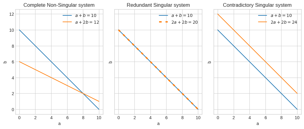
The first system is complete (non-singular) because it has one solution. $a=8$ and $b=2$.

The second system is redundant (singular) because it has many solutions. Any $a$ and $b$ whose sum is 10.

The second system is contradictory (singular) because it has no solutions. No $a+b$ can be equal to 10 while $2(a+b)$ not being 20.

🔑 Singular: peculiar, irregular

🔑 Non-singular: regular

Singularity and linear dependency#

A system of equations can also be represented as lines.

In a non-singular system the lines will intersect at the solution.

In a singular (redundant) system the lines will be one over the other (ie parallel with distant zero).

In a singular (contradictory) system the lines will be parallel and distant from each other.

[2]:

def line1(a):
    return 10.0 - a


def line2(a):
    return 6.0 - (0.5) * a


def line3(a):
    return (20.0 - 2.0 * a) / 2


def line4(a):
    return 12.0 - a


fig, (ax1, ax2, ax3) = plt.subplots(1, 3, figsize=(10, 4), sharex=True, sharey=True)

ax1.plot([0.0, 10.0], [line1(0.0), line1(10.0)], label="$a+b=10$")
ax1.plot([0.0, 10.0], [line2(0.0), line2(10.0)], label="$a+2b=12$")
ax1.set_ylabel("b")
ax1.set_xlabel("a")
ax1.legend()
ax1.set_title("Complete Non-Singular system")
ax1.set_aspect("equal")

ax2.plot([0.0, 10.0], [line1(0.0), line1(10.0)], label="$a+b=10$")
ax2.plot(
    [0.0, 10.0],
    [line3(0.0), line3(10.0)],
    dashes=[2, 3],
    linewidth="3",
    label="$2a+2b=20$",
)
ax2.set_ylabel("b")
ax2.set_xlabel("a")
ax2.legend()
ax2.set_title("Redundant Singular system")
ax2.set_aspect("equal")

ax3.plot([0.0, 10.0], [line1(0.0), line1(10.0)], label="$a+b=10$")
ax3.plot([0.0, 10.0], [line4(0.0), line4(10.0)], label="$2a+2b=24$")
ax3.set_ylabel("b")
ax3.set_xlabel("a")
ax3.legend()
ax3.set_title("Contradictory Singular system")
ax3.set_aspect("equal")

plt.tight_layout()
plt.show()

It turns out that to distinguish between singular and non-singular, the constants can be removed.

Complete	Redundant	Contradictory
$\begin{cases} a + b = 10 \\ a + 2b = 12 \end{cases}$	$\begin{cases} a + b = 10 \\ 2a + 2b = 20 \end{cases}$	$\begin{cases} a + b = 10 \\ 2a + 2b = 24 \end{cases}$

Becomes

Non-Singular	Singular
$\begin{cases} a + b = 0 \\ a + 2b = 0 \end{cases}$	$\begin{cases} a + b = 0 \\ 2a + 2b = 0 \end{cases}$

And this is where the notion of Non-singular and Singular matrices comes in.

Non-Singular	Singular
$\begin{bmatrix} 1 & 1 \\ 1 & 2 \end{bmatrix}$ $\begin{bmatrix} 0 \\ 0 \end{bmatrix}$	$\begin{bmatrix} 1 & 1 \\ 2 & 2 \end{bmatrix}$ $\begin{bmatrix} 0 \\ 0 \end{bmatrix}$

🔑 Singular: the rows are linearly dependent

🔑 Non-singular: the rows are linearly independent

When the rows are linearly independent, there is no constant you can multiply a row by to obtain the second row.

A different interpretation is that each row carries new information that we cannot derive from any other rows.

In contrast, the information provided by the rows of a singular matrix are either redundant or contradictory.

Singularity and the determinant#

🔑 Singular: determinant is zero

🔑 Non-singular: determinant is non-zero

To see how we get to the formula for the determinant and why it’s 0 for singular matrices, let’s consider the matrix $A$.

$A = \begin{bmatrix} a & b \\ c & d \end{bmatrix}$

We saw earlier that $A$ is singular if $(a+b)k = c+d$ for $k > 0$ (linear dependency).

In particular we saw $\begin{bmatrix} 1 & 1 \\ 2 & 2 \end{bmatrix}$ is singular because $(1+1)k = 2+2$ for $k=2$.

Equivalently

$A = \begin{cases} ax + by = 0 \\ cx + dy = 0 \end{cases}$

$=\begin{cases} k_1ax = cx \\ k_2by = dy \end{cases}$

$=\begin{cases} k_1 = \cfrac{c}{a} \\ k_2 = \cfrac{d}{b} \end{cases}$

If $k_1 = k_2 = k > 0$, we obtain

$\cfrac{c}{a} = \cfrac{d}{b}$

We get rid of the fractions and we obtain the formula of the determinant of $A$

$\det A = ad - bc$

$A$ is singular if $ad - bc$ is 0, which implies that $k > 0$

The determinant has the following properties.

🔑 $\det A \times \det B = \det AB$

🔑 $\det A^{-1} = \cfrac{1}{\det A}$

The second one actually can be derived from the first property.

$\det AA^{-1} = \det A \times \det A^{-1}$

$\det I = \det A \times \det A^{-1}$

$\cfrac{\det I}{\det A} = \det A^{-1}$

$\cfrac{1}{\det A} = \det A^{-1}$

Let’s verify the first property, the second property and also that $\det I = 1$

[3]:

A = np.array([[5, 3], [2, 1]])
B = np.array([[1, -1], [3, 4]])

assert np.isclose(np.linalg.det(A) * np.linalg.det(B), np.linalg.det(np.matmul(A, B)))
assert np.isclose(np.linalg.det(np.linalg.inv(A)), 1 / np.linalg.det(A))
assert np.isclose(np.linalg.det(np.linalg.inv(B)), 1 / np.linalg.det(B))
assert np.linalg.det(np.identity(2)) == 1.0

Singularity and rank#

We can think the rank of a matrix in terms of how non-singular a matrix is.

A 2-D matrix has solution in a 2-D space.

When a matrix is non-singular, we get a point as the solution; and since a point has 0 dimensions, the rank is 2.

When a matrix is singular, we get a line as the solution or the whole space. A line has dimension 1 and the whole space has dimension 2, so the rank is 1 and 0, respectively.

Similarly to what we saw for the determinant of matrix, the rank relates to the amount of linearly independent rows of a matrix.

🔑 The rank of a matrix is the number of linearly independent rows

Although this can help develop an intuition of what the rank of a matrix represents, it doesn’t help determine it, especially for large matrices or non-obvious linear dependencies.

One method to determine the rank of a matrix is through the reduced row-echelon form (rref) of a matrix.

Let’s consider the matrix

$\begin{bmatrix}5&&1\\4&&-3\end{bmatrix}$

We can obtain the row echelon form via row operations: - switching any two rows - multiplying (dividing) a row by a non-zero constant - adding (subtracting) one row to another

Row operations are such that they don’t alter the singularity or non-singularity of a matrix, nor its rank.

Divide each row by the leftmost non-zero coefficient

$\begin{bmatrix}1&&\cfrac{1}{5}\\1&&-\cfrac{3}{4}\end{bmatrix}$

Subtract the first row from the second row

$\begin{bmatrix}1&&\cfrac{1}{5}\\0&&-\cfrac{3}{4}-\cfrac{1}{5}\end{bmatrix}$

Divide the last row by the leftmost non-zero coefficient

$\begin{bmatrix}1&&\cfrac{1}{5}\\0&&1\end{bmatrix}$

Multiply the second row by $\cfrac{1}{5}$ and subtract it from the first row

$\begin{bmatrix}1&&0\\0&&1\end{bmatrix}$

Or we can use the rref method of the Matrix data structure from the sp package.

[4]:

sp.Matrix([[5, 1], [1, -3]]).rref(pivots=False)

[4]:

$\displaystyle \left[\begin{matrix}1 & 0\\0 & 1\end{matrix}\right]$

Let’s try to calculate the rref of a singular matrix: a 3x3 matrix where all rows are linearly dependent.

[5]:

sp.Matrix([[1, 2, 3], [3, 6, 9], [2, 4, 6]]).rref(pivots=False)

[5]:

$\displaystyle \left[\begin{matrix}1 & 2 & 3\\0 & 0 & 0\\0 & 0 & 0\end{matrix}\right]$

Let’s try another singular matrix, where only 2 rows are linearly dependent.

[6]:

sp.Matrix([[1, 2, 3], [3, 6, 9], [1, 2, 4]]).rref(pivots=False)

[6]:

$\displaystyle \left[\begin{matrix}1 & 2 & 0\\0 & 0 & 1\\0 & 0 & 0\end{matrix}\right]$

The rref form is characterized by the presence of pivots.

🔑 A pivot is the first non-zero entry of each row in a row-echelon form.

And it turns out the pivots help us determine the rank of a matrix.

🔑 The rank of a matrix is the number of pivots of its row-echelon form

Mathematics for Machine Learning and Data Science

Linear Algebra - Week 1

Contents

Linear Algebra - Week 1#

Singularity#

Singularity and linear dependency#

Singularity and the determinant#

Singularity and rank#